Using Quantum Machine Learning with Amazon Braket to Create a Binary Classifier

By Michael Fischer, Chief of Innovation at Aioi Insurance Services USA, Daniel Brooks, Research Data Scientist formerly of Aioi Insurance Services USA, with AWS quantum solution architects Pavel Lougovski and Tyler Takeshita.

This post details an approach taken by Aioi Insurance Services USA to research an exploratory quantum machine learning application using the Amazon Braket quantum computing service. The term quantum machine learning (QML) has multiple definitions, depending on the context. Here, by QML we mean the use of a quantum computer to perform a machine learning task on classical data. Specifically, we explore how to use quantum computers to build a proof-of-principle binary classifier for risk assessment in a hypothetical car insurance use case. A binary classifier is an algorithm that assigns input data a binary label (0 or 1, Type A or Type B, Safe or Fail, etc.) to “classify” the data. We use a hybrid quantum-classical approach and train a so-called quantum neural network to perform binary classification.

About Aioi

This demonstration is a result of collaboration with Aioi Insurance Services USA — a subsidiary of Aioi Nissay Dowa Insurance which is a member of MS&AD Insurance Group Holdings — a major worldwide insurance organization with close ties to the Toyota group, offering Toyota Insurance in 37 countries. Aioi USA is a full-service “insurtech” insurance agency that develops data science-based products and services for the transportation industry.

Aioi’s Telematics Quantum Machine Learning Use Case

Aioi analyzes telematics data from SAE driving automation L1 and L2 vehicles to predict driving risks. The vehicles are equipped with a multitude of sensors collecting data. Using the data, Aioi would like to assign each vehicle a binary score (safe or fail) that indicates the driving risk score for the vehicle. This risk score assignment task is equivalent to binary classification.

Classical machine learning techniques such as linear regression (LR) or deep learning (DL) have been developed to perform binary classification. LR is a popular approach when the data-label mapping is described by a linear function. For large and complex data structures, DL offers a way to capture nonlinear behavior in data-label mapping.

We already have powerful classical methods to perform classification tasks; so how can quantum computers help here? The short answer is, we don’t quite know yet. The results by Wiebe et al., Phys. Rev. Lett. 109, 050505 (2012) and Schuld et al, Phys. Rev. A 94, 022342 (2016) established that quantum LR algorithms can be exponentially faster than their classical counterparts under the assumption that classical data has been mapped onto a quantum state of a qubit register. The flip side is that these quantum algorithms output a solution in the form of a quantum state which may not be immediately useful for further processing on a classical computer. On the DL front, quantum neural networks (QNNs) emerged as a potential replacement for classical neural nets (Gupta and Zia, Journal of Computer and System Sciences 63, 355–383 (2001)). QNN designs to perform binary classification tasks were proposed recently by Farhi and Neven arXiv:1802.06002 (2018). An advantage of QNNs is that they can directly output a classical label value, though a researcher still has to input data in the form of a quantum state. Whether or not QNNs have practical computational advantage over classical neural nets in DL tasks remains an open question and an area of active research. This motivated us to explore how QNNs can be used for binary classification of binary classical data with an eye towards the constraints imposed by near-term hardware on QNN’s circuit design.

Note, in this post, we build quantum machine learning applications using Amazon Braket. To run the example applications developed here, you need access to the Amazon Braket SDK. You can either install the Braket SDK locally from the Amazon Braket GitHub repo or, alternatively, create a managed notebook in the Amazon Braket console. Please note that you need an AWS account, if you would like to run this demo on one of the quantum hardware backends offered by Amazon Braket.

Setting Up the Quantum Binary Classification Problem

Binary classification is an example of supervised machine learning. It requires a training data set to build a model that can be used to predict labels (driving risk scores). We assume that we are given a training set T that consists of M data-label pairs x, y (T = { x_i , y_i }), i = 1,M . For example, x_i can represent vehicle sensor data as a N-bit string x_i = {x_{i 0} ,…, x_{i N-1} } (x_{i j} = {0,1}), and y_i = {0,1} can represent the driving risk score associated with x_i.

Before we proceed with a quantum solution, it is instructive to recall the main steps of constructing a classical neural net (NN) based solution. A classical NN takes data x and a set of parameters θ₁ ,.., θ_K (so-called weights) as an input and transforms it into an output label Ȳ = f (x, θ₁ ,.., θ_K ) where f is determined by the NN. The goal is then to use a training set to train the NN, i.e. to determine the values of θ₁ ,.., θ_K for which the discrepancy between the output labels and the training set labels is minimized. You achieve this by minimizing a suitably chosen loss function L(Ȳ, y, θ₁ ,.., θ_K ) over the NN parameters θ₁ ,.., θ_K using, for instance, a gradient-based optimizer.

To construct a quantum binary classifier, we follow a similar procedure with a couple of modifications.

We map our classical N-bit data {x_i } onto N-qubit quantum states {|ψ_i〉}. For example, a classical bit string x_i = 0010 maps onto |ψ_i 〉 = |0010〉quantum state.
Instead of a classical NN we construct a QNN, a N+1 qubit circuit C (θ₁ ,.., θ_K ) (a sequence of elementary single- and two-qubit gates), that transforms the input states {|ψ_i 〉|0〉} into output states {|φ_i 〉} such that |φ_i 〉= C |ψ_i 〉|0〉. The QNN circuit C (θ₁ ,.., θ_K ) depends on classical parameters θ₁ ,.., θ_K that can be adjusted to change the output {|φ_i 〉}.
We use the qubit N+1 to read out labels after the QNN acted on the input state. Every time we run the QNN with the same input state and parameters θ₁ ,.., θ_K, we measure in what quantum state the qubit N+1 ends up (|0〉or |1〉). We denote the frequency of observing the state |0〉(|1〉) as p₀ (p₁). We define the observed label Ȳ = (1 – (p₀–p₁))/2. (Note: in the language of quantum computing the difference p₀–p₁ equals the expected value of the Pauli Z operator measured on the qubit N+1). By definition, p₀–p₁ is a function of the QNN parameters θ₁ ,.., θ_K in the range [-1,1] and, thus, Ȳ has the range [0,1].

In the training of the QNN circuit C, our goal is to find a set of parameters θ₁ ,.., θ_K such that for each data point in the training set T, the label value y is close to Ȳ. To achieve this, we minimize the log loss function L(Ȳ, y, θ₁ ,.., θ_K ) defined as:

L(Ȳ, y, θ₁ ,.., θ_K ) = -(∑_iy_ilog(Ȳ_i)+(1-y_i) log(1-Ȳ_i)).

We use the Amazon Braket local simulator that is a part of the Amazon Braket SDK to evaluate L(Ȳ, y, θ₁ ,.., θ_K ) and a classical optimizer from scipy.optimize to minimize it.

1. Mapping Classical Data onto Quantum States

The first step in the implementation of a quantum binary classifier is to specify a quantum circuit that maps classical data onto quantum states. We map classical bit values 0 and 1 onto quantum states |0〉 and |1〉, respectively. By convention, the initial state of a qubit is always assumed to be |0〉. If a quantum algorithm requires the input quantum state to be|1〉, then we obtain it from |0〉 by applying a qubit flip gate X i.e. |1〉 = X |0〉. Below we provide code that generates a quantum circuit for preparing an arbitrary multi-qubit computational basis state|ψ_i 〉 using the Amazon Braket SDK.

# Import Braket libraries
from braket.circuits import Circuit
from braket.aws import AwsDevice

# A function that converts a bit string bitStr into a quantum circuit
def bit_string_to_circuit(bitStr):  
    circuit = Circuit()
    for ind in range(len(bitStr)):
        if bitStr[ind]=='1':
            circuit.x(ind)
            
    return circuit
    
# provide a feature string to test the function above
feature = '11010'

# print quantum circuit that prepares corresponding quantum state 
print(bit_string_to_circuit(feature))

2. Designing the Quantum Neural Network

Now that we know how to prepare input quantum states that correspond to classical data, the next step is to define and construct a QNN circuit C (θ₀ ,.., θ_2N ) that we will train to perform binary classification. We use the QNN design layout depicted in Figure 1 below. It has 2N+1 classical parameters defining: N single-qubit gates R_y(θ_m) acting on qubits m = 0, N-1; one single-qubit gate R_x(θ_N) acting on the qubit N, and N two-qubit gates XX(θ_k) acting on the pairs of qubits {0, n} where n = 1, N.

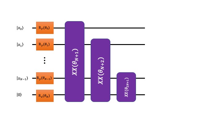
Figure 1. A QNN circuit layout for binary classification. Black horizontal lines represent qubits. Orange and purple boxes represent single- and two-qubit gates respectively. The single-qubit gates R_x and R_y and two-qubit gates XX are standard gates defined in Amazon Braket SDK.

The code below implements this QNN, applies it to an arbitrary input state defined by a classical bit string, and measures the values of the label qubit.

# import standard numpy libraries and optimizers
import numpy as np
from scipy.optimize import minimize

# Braket imports
from braket.circuits import Circuit, Gate, Instruction, circuit, Observable
from braket.aws import AwsDevice, AwsQuantumTask
from braket.devices import LocalSimulator

# set Braket backend to local simulator (can be changed to other backends)
device = LocalSimulator() 

# Quantum Neural Net from the QNN figure implemented in Braket
# Inputs: bitStr - data bit string (e.g. '01010101')
#         pars - array of parameters theta (see the QNN figure for more details) 

def QNN(bitStr,pars):
    ## size of the quantum neural net circuit
    nQbts = len(bitStr) + 1 # extra qubit is allocated for the label 
    
    ## initialize the circuit
    qnn = Circuit()
    
    ## add single-qubit X rotation to the label qubit, 
    ## initialize the input state to the one specified by bitStr
    ## add single-qubit Y rotations to data qubits, 
    ## add XX gate between qubit i and the label qubit, 
    qnn.rx(nQbts-1, pars[0])
    for ind in range(nQbts-1):
        angles = pars[2*ind + 1:2*ind+1+2]
        if bitStr[ind] == '1': # by default Braket sets input states to '0', 
                               # qnn.x(ind) flips qubit number ind to state |1\ 
            qnn.x(ind)
        qnn.ry(ind, angles[0]).xx(ind, nQbts-1, angles[1])
    
    ## add Z observable to the label qubit
    observZ = Observable.Z()
    qnn.expectation(observZ, target=[nQbts-1]) 
    
    return qnn

3. Training the Quantum Neural Network

With the QNN defined, we need to code up the loss function L(Ȳ, y, θ₁ ,.., θ_K ) that we minimize in order to train the QNN to perform binary classification. Below is the code that computes L(Ȳ, y, θ₁ ,.., θ_K ) using the local simulator in Amazon Braket.

## Function that computes the label of a given feature bit sting bitStr

def parity(bitStr):
    return bitStr.count('1') % 2

## Log loss function L(theta,phi) for a given training set trainSet
## inputs: trainSet - array of feature bit strings e.g. ['0101','1110','0000'] 
##         pars - quantum neural net parameters theta (See the QNN figure)
##         device -  Braket backend that will compute the log loss
def loss(trainSet, pars, device):
    loss = 0.0
    for ind in range(np.size(trainSet)):  
        ## run QNN on Braket device
        task = device.run(QNN(trainSet[ind], pars), shots=0) 
        ## retrieve the run results <Z>
        result = task.result()
          
        if parity(trainSet[ind])==0:
            loss += -np.log2(1.0-0.5*(1.0-result.values[0]))
        else:
            loss += -np.log2(0.5*(1.0-result.values[0]))
    print ("Current value of the loss function: ", loss)
    return loss

Putting it all together, we are now ready to train our QNN circuit to reproduce binary classification of a training set T. For the example below, we assume that labels y_i are generated by a Boolean function F(x_i) = (∑_j x_ij) mod 2. To emulate data in the training set T, we generate eleven random 10-bit strings (data) and assign them labels according to F.

## Training the QNN using gradient-based optimizer
nBits = 10 # number of bits per data string

## Random training set consisting of 11 10-bit data strings
## Please explore other training sets
trainSet = ['1101011010',
            '1000110011',
            '0101001001',
            '0010000110',
            '0101111010',
            '0000100010',
            '1001010000',
            '1100110001',
            '1000010001',
            '0000111101',
            '0000000001']

## Initial assignment of QNN parameters theta and phi (random angles in [-pi,pi]) 
pars0 = 2 * np.pi * np.random.rand(2*nBits+1) - np.pi

## Run minimization
res = minimize(lambda pars: loss(trainSet, pars, device), pars0, method='BFGS', options={'disp':True})

Run the code above and wait for the optimizer to converge. It outputs a message that looks like this when the optimizer finishes.

Optimization terminated successfully.
         Current function value: 0.000000
         Iterations: 55
         Function evaluations: 1430
         Gradient evaluations: 65

We note that our QNN circuit is designed to compute the parity of input data exactly for an appropriate choice of the parameters θ₀ ,.., θ_2N. Thus, the global minimum of the loss function using this QNN is zero. This is generally not the case in DL applications, however. Note also that L(Ȳ, y, θ₀ ,.., θ_2N ) is not convex with respect to the parameters θ₀ ,.., θ_2N. This means that if the final value of the loss function value is not zero, the optimizer got stuck in a local minimum. Do not panic. Try running the optimizer with a different set of initial parameters pars0. You can also explore various minimization algorithms by specifying method=' ' in the minimize function.

Calling res.x outputs the optimal values of the parameters θ₀ ,.., θ_2N, and you can use them to run the “optimal” QNN and perform binary classification on the data that is not a part of the training set. Try that and compute the mean squared error of the classifier.

There are 1024 possible 10-bit strings. For our example, we chose a training set that has only 11 data points (bit strings). Yet it is sufficiently large to train the QNN to act as a perfect binary classifier for all 1024 possible features. Let’s demonstrate that.

## Print the predicted label values for all N-bit data points using the optimal QNN parameters res.x
for ind in range(2**nBits):
    data = format(ind, '0'+str(nBits)+'b')
    task = device.run(QNN(data, res.x), shots=100)
    result = task.result()
    if (data in trainSet):
        inSet = 'in the training set'
    else:
        inSet = 'NOT in the training set'
    print('Feature:', data, '| QNN predicted parity: ', 0.5*(1-result.values[0]), ' | ', inSet) 
    print('---------------------------------------------------')

As an exercise, use the optimal QNN parameters in res.x and apply the resulting QNN to all 10-bit strings that are not in the training set. Record the mean squared error between the predicted and computed label values.

Conclusion

Predicting driving risk scores for L1 and L2 driving automation vehicles is a computational task poised to become a mainstay as vehicle driving automation increases to L3, L4 and L5. The problem amounts to binary classification. Classical machine learning techniques such as DL can be applied to solve the problem. But can the emerging quantum computing technology solve this problem as well? This post explored how quantum machine learning can also be used to perform binary classification and analyze binary (telematics) data by combining QNNs with the Amazon Braket quantum computing service. The QNN binary classifier designed in this post has a number of quantum gates that scales linearly with the size of each data point. This is advantageous for implementation on near-term quantum computers that are currently limited in the number of sequential quantum gates they can support. A future area of investigation for the team at Aioi is to apply more complex data sets, and constructing QNNs to classify them. You can explore or try out the code from this post on Github.

The content and opinions in this post are those of the third-party author and AWS is not responsible for the content or accuracy of this post.

AWS Quantum Technologies Blog