AWS Quantum Technologies Blog
Noise in Quantum Computing
Customers looking to solve their hardest computational problems often wonder about the production-readiness of quantum computing. They want to know when a full-scale, fault-tolerant quantum computer will be available, and what the obstacles are to achieving this ambitious goal. Current generation quantum computers are not fault-tolerant and have limited utility, but customers are experimenting with the effects of realistic errors in their quantum algorithms in what we call “noisy” quantum devices. Amazon Braket enables you to experiment by providing access to quantum simulators that can reproduce the effects of noise and errors.
In this blog, we introduce the concept of noise in quantum computing, and we take a practical approach to describing how noise affects qubits in a computation. We also show how you can build custom noise channels using the density matrix simulators available in Amazon Braket.
What is noise?
Noise refers to the multiple factors that can affect the accuracy of the calculations a quantum computer performs. Quantum computers are susceptible to noise from various sources, like disturbances in Earth’s magnetic field, local radiation from Wi-Fi or mobile phones, cosmic rays, and even the influence that neighboring qubits –the building blocks of a quantum computer– exert on each other by mere proximity. These disruptions cause the information an idle qubit holds to fade away. Lastly, when performing a quantum logic operation, qubits can also suffer from errors that cause them to rotate by the wrong amount. In all cases, the final state of the quantum computer is not precisely the state one expects. Unless one can reverse the action of the noise, the information in the quantum system can become randomized or totally erased. This phenomenon is known as decoherence.
Since quantum information is highly prone to decoherence, the outlook for quantum computing appears bleak at first. Fortunately, a beautiful technique known as quantum error correction (QEC) provides a path forward: information is carefully and redundantly encoded into multiple qubits such that the effects of noise on the system can be, as the name suggests, corrected. QEC is a rich subject, but a key difficulty to reaching full fault-tolerant quantum computing (wherein the probability of logical errors can be made arbitrarily small) is that current schemes require a large overhead in the total number of qubits.
In addition to researching quantum error correction, AWS customers are also looking for ways to do more with less by studying applications of currently available noisy, intermediate-scale quantum (NISQ) devices. It is an open question whether or not we will be able to find quantum advantage using NISQ devices, but groups in academia and industry have been developing algorithms that nevertheless get the most performance out of current quantum computers, which are limited by their size and coherence. Researchers evaluate these algorithms in the presence of noise to understand how well near-term devices can perform in realistic scenarios. Noise simulation provides a systematic approach to evaluating noisy algorithms by making it possible to choose between different types of noise with tunable strength.
As quantum hardware efforts advance, researchers are keen to understand the way noise affects new devices by modeling errors and running noisy simulations with these error models. By comparing noisy simulations with hardware measurements, experimenters can characterize the noise in new hardware, informing future hardware advances, algorithm design, and quantum error correction research.
An introduction to noise simulation
The Schrödinger equation describes the evolution of a quantum state over time, by way of unitary operators acting on the state. In a quantum computer, these unitary operators can be precisely controlled, giving rise to a set of logical gates for transforming the quantum state of the computer. Logic gates are the building blocks of quantum circuits, and they operate on one or several qubits. While these gates drive the evolution of so-called pure quantum states, they cannot describe noisy quantum evolution, decoherence, or open quantum systems. To model these things, a richer description of quantum states and quantum operations is needed, which we will describe in a later section.
In the code snippet that follows, the quantum computer is instructed to produce a Bell pair, in which a pair of qubits is maximally entangled. In the computational basis:
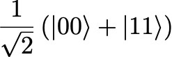
In a noiseless setting, measurements of this state would produce measurement outcomes of 00 and 11 with equal probability. However, in a noisy setting, the quantum computer can give erroneous results. Indeed, as observed in the measurement counts below, we find 01 and 10 bitstrings, along with the 00 and 11 results we expected. In fact, in this example, the states 01 and 10 represent 9.5% of the total results:
from braket.circuits import Circuit, Gate
from braket.aws import AwsDevice
from matplotlib import pyplot as plt

# set up device
rigetti = AwsDevice("arn:aws:braket:us-west-1::device/qpu/rigetti/Aspen-M-2")

# create a maximum entangled state.
bell = Circuit().h(0).cnot(0, 1)

# run circuit
rigetti_task = rigetti.run(bell, shots=1000)

# get measurement counts
rigetti_results = rigetti_task.result()
rigetti_counts = rigetti_results.measurement_counts
print('Measurement counts:', rigetti_counts)

# plot results: see effects of noise
%matplotlib inline
plt.bar(rigetti_counts.keys(), rigetti_counts.values())
plt.xlabel('bitstrings')
plt.ylabel('counts')
plt.tight_layout()
Output:
Measurement counts: Counter({'00': 463, '11': 442, '10': 60, '01': 35})
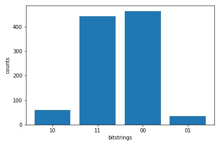
Figure 1: Results of a Bell circuit run on noisy quantum hardware, highlighting the effects of the noise.
How can this be? The answer is that noise corrupted the quantum information in the device, leading to the unexpected measurement results. The example above highlights the reality of all NISQ devices: they are prone to errors in the computation. In order to simulate the (noisy) evolution in NISQ hardware, we need a quantum simulator that can model general noise acting on the quantum circuit.
Density matrices
Since our goal is to model a wide variety of both pure and noisy quantum operations, we require a richer representation of quantum states than just state vectors and quantum circuits. What we really need are so-called mixed quantum states, which are required when we want to describe, for example, a physical system that is subject to noise and decoherence, or is entangled with other quantum systems in the environment outside of our control.
Mathematically, the more general description of quantum states we need makes use of “density matrices” to describe both pure and mixed quantum states. For pure quantum states, the state vector formalism and the density matrix formalism coincide: for each pure state |ψ⟩, there is a density matrix ρ=|ψ⟩⟨ψ| (the outer product of the state |ψ⟩ and its conjugate transpose) that are equivalent representations of the same state. The density matrix formalism allows for more general quantum states than the pure states, and indeed mixed states can be represented by taking convex combinations of pure state density matrices: ρ=∑i si |ψi⟩⟨ψi| with trρ=1.
The beauty of the density matrix formalism is that it encompasses both pure and mixed states, which allows us to simulate more general processes in nature that involve noise and incomplete information. For example, a qubit in the |0⟩ state that undergoes a bit flip error with probability s evolves from a (pure state) density matrix ρ=|0⟩⟨0| to a mixed state ρ’=(1-s)|0⟩⟨0|+s|1⟩⟨1|. This final density matrix is a mixed state representing a qubit that is either in |0⟩ or |1⟩ with a probability distribution {(1-s), s}. This density matrix represents an incoherent mixture of |0⟩ and |1⟩, rather than a coherent superposition.
With density matrices in hand, we are now equipped to describe general types of operations that can be applied to a quantum system, known as quantum channels. We can accurately model noisy quantum dynamics and decoherence with quantum channels.
Quantum Channels and the Kraus representation
A quantum channel is a general operation on a quantum state. Until May 2021, Amazon Braket customers could only create quantum circuits that were composed of gates and unitary transformations, but not general quantum channels. There are, however, more general transformations that one can perform on a quantum state, such as adding noise, or evolving to a mixed state. With the advent of the On-Demand Density Matrix simulator (DM1) and the local density matrix simulator, Amazon Braket enables customers to simulate these more general transformations and states.
Mathematically, quantum channels are completely positive, trace-preserving maps that act on density matrices. To represent quantum channels mathematically, we use the Kraus decomposition, also known as the operator-sum representation. A quantum channel ? acting on a density matrix ρ can be decomposed as ?(ρ) = ∑i si Ki ρi Ki†, where the Ki are Kraus operators describing the quantum channel, and the si are the probabilities associated with applying Ki, i.e., si is the probability that the operator represented by the Kraus operator Ki occurs. Let’s consider some examples:
Example 1: Unitary gates. Consider a unitary U acting on a state |ψ⟩, which gives us a new state |ϕ⟩ = U|ψ⟩. In the density matrix formalism, we can see straight away that ρ’ := |ϕ⟩⟨ϕ| = U|ψ⟩⟨ψ|U† = UρU†. Thus, for a unitary gate U, the associated quantum channel is given by ρ’ = ?U(ρ) = UρU†. In this case, there is only one Kraus operator (i.e., K1 = U), and it is applied with probability s1 = 1.
Example 2: Bit flip error. Consider again a single qubit undergoing bit flip noise that flips the state between 0 and 1 with probability s. We stated earlier that if the qubit begins in the state |0⟩⟨0|, then the final state is given by ρ’ = (1-s)|0⟩⟨0| + s|1⟩⟨1|. More generally, the quantum channel associated with bit flip errors is given by ?bit flip = (1-s)ρ + sXρX, where X is a Pauli matrix. In this form, we can immediately read off the Kraus operators for the channel: K1=I (the identity), and K2 = X (a bit flip), which are applied with probabilities (1-s) and s, respectively. Intuitively, this makes sense: with probability s, we flip the bit (by applying an X gate), and with probability (1-s) we do nothing. If we set ρ = |0⟩⟨0|, we can confirm that we arrive at the final state ρ’ above.
Difference between SV1 and DM1 simulators
Amazon Braket’s state vector simulator, SV1, represents the quantum state as a state vector describing a pure state. If we want to simulate arbitrary noise, we need to use density matrices. DM1 represents the quantum state as a density matrix, with the advantage that common noise quantum channels[1] are predefined in the Amazon Braket SDK, so you do not need to manually define Kraus operators for these channels. You can simply add the predefined channels to a circuit, and DM1 will simulate the circuit with noise.
There is also a difference in capacity between SV1 and DM1. While SV1 supports 34 qubits, the maximum number of qubits supported by DM1 is 17. This is due to the additional memory requirement of storing a density matrix compared to a state vector. On the other hand, both simulators come with a maximum runtime of 6 hours and allow up to 50 concurrent tasks.
Local and hosted Amazon Braket noise simulators
Amazon Braket provides two density matrix simulators: a local simulator (braket_dm) that comes with the Braket SDK, and an On-Demand Density Matrix simulator (DM1).
The local simulator is convenient for fast prototyping, and there is no requirement for you to have access to an AWS account. The local density matrix simulator[2] comes preinstalled with the Amazon Braket SDK, and it can be instantiated using the parameter 'braket_dm' that is passed when declaring the local simulator:
from braket.devices import LocalSimulator
device = LocalSimulator('braket_dm')
Using the local simulator has limitations on the circuit depth and size that can be defined, as they are determined by the available resources on the local machine. The local simulator can run circuits with noise up to 12 qubits without any concurrency. For larger experiments, a better option is to use the On-Demand DM1 simulator[3]. This is defined using its corresponding Amazon Resource Name (ARN):
from braket.aws import AwsDevice
device = AwsDevice("arn:aws:braket:::device/quantum-simulator/amazon/dm1")
See the Developer Guide[4] to learn more about how to choose a simulator for your workload based on your requirements.
Types of noise
Before building a noisy circuit, let’s cover the different types of noise that are readily implemented in Amazon Braket. The following list shows the most commonly used 1- and 2-qubit noise channels in simulations. These channels are predefined in the Amazon Braket SDK and can be directly applied to circuits.
Bit flip: When measured in the computational state, the qubit flips from |0⟩ to |1⟩ or vice versa with some specified probability. Bit flip errors are modeled by applying an X gate. The Kraus representation is ?(ρ) = (1-s)ρ + sXρX, where s is the probability of a bit flip error.
Phase flip: This error affects the phase of the qubit, rotating around the Z axis, mapping |1⟩ to –|1⟩. Phase flip errors are modeled by applying a Z gate. The Kraus representation is ?(ρ) = (1-s)ρ + sZρZ, where s is the probability of a phase flip error.
Depolarizing: This channel describes the process in which a 1-qubit quantum state loses its quantum information and decays into an incoherent mixture of the computational basis states, |0⟩⟨0| or |1⟩⟨1|. The quantum state loses the phase as well as the superposition between basis states. The Kraus representation is ?(ρ) = (1-s)ρ + s/3 (XρX + YρY + ZρZ), where s controls the strength of the noise.
Amplitude damping: This channel models the asymmetric process through which the qubit state |1⟩ irreversibly decays into the state |0⟩. As an example, in a quantum computer, the state |1⟩ could have a higher energy than state |0⟩, and while qubits are designed such that both |0⟩ and |1⟩ have long lifetimes, the system can still decay from |1⟩ to the lower energy state |0⟩. The Kraus representation is ?(ρ) = K1ρK1† + K2ρK2†, with K1 = [1,0;0,√1-s], K2 = [0,√s;0,0], and s is the probability of decay.
Pauli channel: In Pauli channels, Kraus operators are constructed out of Pauli matrices. You can define a general noise channel with the probabilities of Pauli X, Y and Z matrices, respectively, as Kraus operators. The Kraus representation is ?(ρ) = (1 – sx – sy – sz)ρ + sxXρX + syYρY + szZρZ, with sx, sy, and sz being the probability of each Pauli error.
Two-qubit depolarizing: This channel describes the process under which a 2-qubit quantum state undergoes depolarizing noise, as above. The state loses its quantum phase as well as the superposition between basis states. The Kraus representation is ?(ρ) = ∑i si KiρKi†, where Ki is one of the sixteen two-qubit Pauli matrices and s is the probability of the corresponding Ki.
Two-qubit dephasing: This channel describes the process under which a 2-qubit quantum state undergoes dephasing noise, as above. The Kraus representation is ?(ρ) = (1-s)ρ + s/3 (IZρIZ + ZIρZI + ZZρZZ), where s is the strength of the noise.
For more details on the Kraus representation and specific parameters of these channels, refer to the Simulating Noise in Amazon Braket[1] notebook.
Applying noise to the whole circuit vs. individual gates and qubits
Just as we can build a noiseless circuit with quantum gates, we can build a noisy quantum circuit from the bottom up. In the following example, we start with the Bell pair preparation circuit seen previously, and to it we add a noise channel right after each gate: a bit flip and a phase flip with probability values of 0.1:
from braket.circuits import Circuit
circuit = Circuit().h(0).bit_flip(0,0.1).cnot(0,1).phase_flip(0,0.1)
We can also use the apply_gate_noise method to add noise channels to a circuit. For example, to add noise to every gate in a circuit, we can define it separately and then apply it to the whole circuit:
from braket.circuits import Circuit, Noise
circuit = Circuit().h(0).cnot(0,1)
noise = Noise.BitFlip(probability=0.1)
circuit.apply_gate_noise(noise)
Finally, it is possible to add noise to a particular gate or a particular qubit individually. The following example uses the keyword argument target_qubits in apply_gate_noise to add noise1 to all gates for qubit 1, and target_gates to add noise2 to all the H gates in the circuit.
from braket.circuits import Circuit, Noise, Gate
circuit = Circuit().h(0).cnot(0,1)
noise1 = Noise.BitFlip(probability=0.1)
noise2 = Noise.PhaseFlip(probability=0.2)
circuit.apply_gate_noise(noise1, target_qubits=[1])
circuit.apply_gate_noise(noise2, target_gates=[Gate.H])
See the Developer Guide[5] to learn more about constructing circuits with noise channels.
Custom noise channels
In certain situations, it may make more sense to define a custom noise channel. For example, one may want to simulate the behavior of a special quantum system that produces a type of noise that cannot be directly composed using the predefined noise channels. In this case, it is possible to define noise channels with a list of Kraus operators. Each Kraus operator is represented by a matrix defined by the customer. The dimension of each matrix must agree with the number of qubits on which the custom noise channel acts. For example, the matrix must be 2×2 for 1-qubit noise, and 4×4 for 2-qubit noise:
from braket.circuits import Noise
import numpy as np

K0 = np.array([[1, 1], [1, 1]]) * 0.5
K1 = np.array([[1, -1],[-1, 1]]) * 0.5
noise = Noise.Kraus([K0, K1])
Example: Bit flip error correction (repetition code)
One of the uses of noise simulation is quantum algorithm research. As an example, we can evaluate the repetition bit flip error correction code[6], which is designed to resist bit flip noise by encoding a logical qubit into three physical qubits. The following code snippet shows how one would test this code.
from braket.circuits import Circuit, Noise
from braket.devices import LocalSimulator
from braket.aws import AwsDevice

# step 1: prepare an initial state
circuit = Circuit().x(0)

# step 2: apply bit flip code
circuit.cnot(0,1).cnot(0,2)

# step 3: add noise to the circuit
for i in range(3):
     circuit.bit_flip(i,0.1)

# step 4: error correction
circuit.cnot(0,1).cnot(0,2).ccnot(1,2,0)

# measure the probability of qubit 0
circuit.probability(0)
We first initialize the first qubit q0 into the state we wish to encode. We then encode this information by applying two CNOT gates to entangle qubit 0 with qubits 1 and 2. The encoding redundantly stores the initial state on qubit 0 across all three qubits. If any of one of the three qubits undergoes a bit flip error, we can still recover the initial state by decoding the information. In practice, this is done by checking the parity between the different qubits, which tells us which qubit underwent a bit flip error, but without revealing or disturbing the encoded information. The full process is shown in Figure 2. Let us test this QEC scheme using a noise simulation. We will choose our initial state to be |1⟩, apply a bit flip noise to all three qubits, and then apply the error correction step before reading out.
# Use this line to run the local density matrix simulator
dev = LocalSimulator("braket_dm")

# Use this line to run the managed density matrix simulator DM1
dev = AwsDevice("arn:aws:braket:::device/quantum-simulator/amazon/dm1")

task = dev.run(circuit, shots=100)
print(task.result().values)
Output:
[array([0.02, 0.98])]
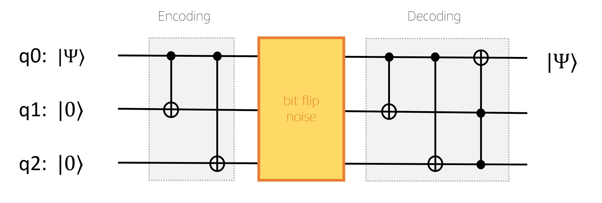
Figure 2. Schematic circuit representation of bit flip error correction, tested using simulated noise on all three qubits.
We can choose to run this circuit on a local simulator or on DM1. Refer to the Developer Guide[4] to learn how to choose a simulator for your workload based on your requirements. After running the circuit on a density matrix simulator, the probability distribution of qubit 0 is [0.02, 0.98]. This distribution indicates that 98% of the circuit executions measure qubit 0 to be in the |1⟩ state. In other words, the error rate is 2%, which is a reduction from the 10% noise rate of the bit flip error. This repetition code is able to correct up to one bit-flip error in the circuit, but not two or more bit-flips. The 2% error rate we see accounts for these cases, in which more than one qubit underwent a bit flip error. To drive this point home, if we skip step 2 and step 4 (i.e., skipping the error correction) the results are [0.11, 0.89], which is more in line with our 10% error rate.
Simulate quantum hardware behavior
The examples shown so far allow for simulations with arbitrarily chosen parameters, being up to the researcher to decide which noise to choose, how often, and where (initialization, per-qubit, per-gate, or readout). Another use case for the noise simulator is the ability to model real quantum hardware. The Amazon Braket console shows calibration data for each quantum processing unit (QPU) detailing the fidelity of the physical qubits and native gates on the hardware. This information is also available via the GetDevice method in the Amazon Braket SDK. By extracting the relevant values from this calibration data, it is possible to construct a noise model that approximates the real behavior of the quantum device.
In the following example, we use the initial Bell pair running on Rigetti’s Aspen-M-2 QPU, and we build a circuit that emulates the real noise that one would encounter by running the Bell circuit on the actual QPU.
To have better control of what gates are executed, we use verbatim compilation in combination with natively supported gates by Rigetti. Verbatim mode effectively turns off compilation in the backend so that the gates passed to the QPU are the same gates executed in the hardware, without decomposing or modifying the circuit. Refer to this example notebook to learn more about verbatim compilation[7].
A Bell circuit consists of a single-qubit Hadamard gate, and a two-qubit CNOT gate. In order to decompose this circuit into hardware-native gates for Rigetti, we will decompose the Hadamard and CNOT gates into their equivalent low-level (native) rotations. We first check the native gates supported by Rigetti:
# Define the device
device = AwsDevice("arn:aws:braket:us-west-1::device/qpu/rigetti/Aspen-M-2")

# Print its native gates
print('Supported gateset: \n', device.properties.paradigm.nativeGateSet)
Output:
Supported gateset:
['rx', 'rz', 'cz',
'cphaseshift', 'xy']
We now rewrite the original circuit using the native gates above, and also activate verbatim mode by using a “verbatim box” within the circuit definition. An additional feature we use here is disable_qubit_rewiring flag to True, so we get to select which qubits we want our circuit to run on. In this example we have selected qubits 36 and 37:
import math
pi = math.pi

q1 = 36
q2 = 37

# Bell pair decomposition into native gates
circuit = Circuit().rz(q1,pi/2).rx(q1,pi/2)
circuit = circuit.rz(q2,-pi/2).rx(q2,pi/2)
circuit = circuit.cz(q2,q1)
circuit = circuit.rx(q2,-pi/2).rz(q1,-pi/2).rz(q2,-pi/2)

circuit = Circuit().add_verbatim_box(circuit)
task = device.run(circuit, shots=1000, disable_qubit_rewiring=True)
To perform noise simulation for the above circuit, we first retrieve calibration data for the hardware, as it contains the needed information about noise, such as gate and readout fidelities. This example notebook[8] shows how one can retrieve hardware properties, including the calibration data. We can retrieve the calibration data with the properties.provider command.
Secondly, we need to decide how to model noise in the circuit, i.e., what type of noise is associated with the calibration and what is the noise rate. Accurately modelling noise in hardware is an active field of research, but in this example, we use a simple noise model that considers both gate noise and readout noise.
Depolarizing noise is the process by which the quantum information in a state is lost, and the state degrades into just classical state (e.g., a basis |0⟩ or |1⟩ state). In lieu of a detailed noise model for the Rigetti device, we can simply model the noise with a depolarizing noise channel, which captures both bit flip and phase flip errors, and is a good model for an unknown quantum channel. In this example, we use single qubit depolarization to model noise that affects the 1-qubit gates, and 2-qubit depolarizing noise for 2-qubit gate. Finally, readout noise is the process in which |0⟩ is reported as 1, and |1⟩ is reported as 0. To model readout noise, we use the bit flip channel with a noise probability equal to the readout error rate.
from braket.circuits import Circuit, Gate, Noise
from braket.devices import LocalSimulator
from braket.aws import AwsDevice

# Define the device
device = AwsDevice("arn:aws:braket:us-west-1::device/qpu/rigetti/Aspen-M-2")

q1 = 36
q2 = 37
calibration1Q = device.properties.provider.specs['1Q']
calibration2Q = device.properties.provider.specs['2Q']

circuit = Circuit().rz(0,pi/2).rx(0,pi/2)
circuit.rz(1,-pi/2).rx(1,pi/2)
circuit.cz(1,0)
circuit.rx(1,-pi/2).rz(0,-pi/2).rz(1,-pi/2)

depolar_rate_1Q_q1 = 1 - calibration1Q[f'{q1}']["f1QRB"]
noise1Q_q1 = Noise.Depolarizing(probability=depolar_rate_1Q_q1)

depolar_rate_1Q_q2 = 1 - calibration1Q[f'{q2}']["f1QRB"]
noise1Q_q2 = Noise.Depolarizing(probability=depolar_rate_1Q_q2)

depolar_rate_2Q = 1 - calibration2Q[f'{q1}-{q2}']["fCZ"]
noise2Q = Noise.TwoQubitDepolarizing(probability=depolar_rate_2Q)

circuit.apply_gate_noise(noise1Q_q1, target_gates=[Gate.Rx, Gate.Rz], target_qubits=0)
circuit.apply_gate_noise(noise1Q_q2, target_gates=[Gate.Rx, Gate.Rz], target_qubits=1)
circuit.apply_gate_noise(noise2Q, target_gates=Gate.CZ)

readout_rate0 = 1 - calibration1Q[f'{q1}']["fRO"]
readout_rate1 = 1 - calibration1Q[f'{q2}']["fRO"]
circuit.apply_readout_noise(Noise.BitFlip(probability=readout_rate0), target_qubits=0)
circuit.apply_readout_noise(Noise.BitFlip(probability=readout_rate1), target_qubits=1)

dev = LocalSimulator("braket_dm")
task = dev.run(circuit, shots=1000)
count_simulator = task.result().measurement_counts
With the noisy circuit we just created, we can now perform the noise simulation. The result is shown in the figure below.
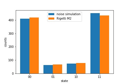
Figure 3. Side-by-side outcome of a Bell pair run on the DM1 simulator (blue) and Rigetti Aspen-M quantum device (orange).
The distribution from noise simulation follows the trend of the hardware measurement, suggesting that our simple noise model consisting of only depolarizing noise is a good approximation to the true noise model in the device. The difference between the simulation and the measurement comes from several factors. Firstly, the measurement counts are a statistical sampling of the quantum state. Even if the underlying quantum state is the same, there will be statistical variation in the sampling. Secondly, the hardware calibration data is only measured periodically, usually at least once a day. It is possible that the hardware noise properties drift from those that were measured in the last calibration and reported by the device. In addition, the way the noises are modeled can greatly impact the quality of the simulation. The simple depolarizing model chosen above works well because commonly occurring noise sources have an expected effect that is accurately modeled by depolarizing noise. However, the presence of exotic and more complex noise in the behavior of the device might not be well captured by a simple noise model. The effect of these factors can be quantified with a more detailed numerical analysis, which is beyond the scope of this blog.
In the above example, we import the noise properties from the hardware and then add noise channels to the Bell circuit based on a simple noise model that only has depolarizing noise and readout noise. If a more advanced noise model is desired, or if it needs to be applied to many circuits, one can create a NoiseModel class that allows for custom rules that determine how and when noise channels are added to quantum circuits. See this example notebook[9] to get started with building your very own noise model.
Conclusion
In this blog, we learned how to create a circuit with predefined noise channels on Amazon Braket, such as the bit-flip and phase-flip channels, or custom noise channels for noise simulations. Not only can you write the noisy circuit from bottom up, you can also add noise channels to a circuit that you have already created. We learned that a density matrix simulator is required to perform noise simulations, and that one can use Amazon Braket local or on-demand density matrix simulators. To get started and dive deeper, see our example notebooks on the topic of creating and simulating noisy circuits[1] and simulating noise using the noise profile of a piece of hardware[10].
References
[1] Notebook: Simulating Noise On Amazon Braket
[2] Local density matrix simulator (braket_dm)
[3] Density matrix simulator (DM1)
[4] Developer Guide: Compare simulators
[5] Developer Guide: Noise simulation
[6] Bit flip code
[7] Notebook: Verbatim compilation
[8] Notebook: Getting Devices and Checking Device Properties
[9] Notebook: Noise models on Rigetti Aspen M2
[10] Noise models