AWS HPC Blog
Using machine learning to drive faster automotive design cycles
The automotive product engineering process involves months or years of iterative design reviews and refinement, with back-and-forth feedback between stakeholders regularly to adjust designs and evaluate the impact of design changes on engineering metrics like the coefficient of drag. Between each design iteration, engineers wait hours or days for simulations to complete, which means they can only execute a handful of design decisions each week.
In this post, we’ll show how automakers can reduce cycle times from hours to seconds by leveraging surrogate machine-learning (ML) models in place of HPC, physics-based simulations and create subtle design variations for non-parametric geometries.
In short: automotive engineers can use emerging ML methodologies to speed up the product engineering process.
Background
Typically, the automotive product design process involves conceptualization, computer-aided design (CAD) geometry creation, and engineering simulations for validating the designs to ensure aerodynamic efficiency and desired structural stability.
Recent advances in AI/ML and Generative AI technology including algorithms such as MeshGraphNets, U-Nets and Variational Autoencoders, have provided a path towards accelerating the design process through fast ML inferences which allow us to run fewer full-fidelity physics-based HPC simulations, which can take hours, while gathering insight into large design spaces.
In this work, we’ll focus on computational fluid dynamics (CFD) simulations for intelligent aerodynamic surface design, though there are often other design considerations like impact response, noise, vibration and harshness.
The goal of this work is not to develop a comprehensive toolkit for aerodynamic design – we want to present a simple user experience to show how engineers can use scientific ML methods, together with AWS services to deliver business value. We’ll mainly use AWS Batch, Nice DCV, Amazon S3 and Amazon SageMaker. We’ll also explain how to build a web application that uses ML and generative design to enhance these development processes.
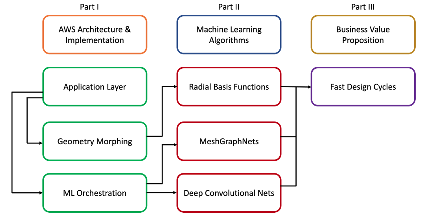
Figure 1 – Overview of Workflow Structure incorporating Web Application UI overview, AI/ML Methodology and AWS Implementation
Roadmap for this post
Much like the workflow chart in Figure 1, we’ll divide this post into three parts.
First, we’ll start by explaining how to build a minimally viable web application including the end user experience and core components starting from an AWS architecture blueprint, highlighting some key components.
Next, we’ll dive deep into the underlying ML models including the training methodology and inference deployment.
Finally, we’ll wrap up with a brief discussion about how we imagine automakers using workflows like this in practice to augment and accelerate the product design lifecycles.
Cloud implementation and AWS architecture
Let’s look at how to quickly and securely implement a minimally-viable web application. Using that, we’ll generate ground truth meshes, run OpenFOAM simulations, and train the machine learning models using AWS HPC services.
AWS architecture. We don’t want to completely replace HPC simulations – these are necessary for verification and validation. We want to enable engineers to quickly build a web application inside their environment, access it securely, and store all their related artifacts. For this reason, we’ve chosen a minimalist architecture and we’ll leave it up to the automaker to decide how to integrate this into their existing environment.
Figure 2: AWS Architecture diagram for deployment on a g5 instance using DCV, with endpoints to retrieve data or optionally submit compute jobs on self-managed ML endpoints (AWS Batch) or Amazon SageMaker
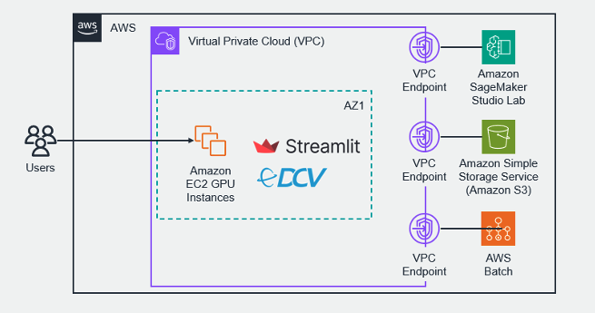
Figure 2: AWS Architecture diagram for deployment on a g5 instance using DCV, with endpoints to retrieve data or optionally submit compute jobs on self-managed ML endpoints (AWS Batch) or Amazon SageMaker
We’re hosting the web application on a g5.12xlarge Amazon Elastic Compute Cloud (Amazon EC2) instance. The G5 has 4 x A10G NVIDIA GPUs to serve the machine learning models and we’re using the NICE DCV streaming protocol to securely stream the desktop to the end.
We’re also keeping the EC2 instance secure inside of a VPC and we only allow TCP traffic to flow from the instance to a single end user.
We train drag prediction models using Amazon SageMaker, and we securely store the inputs and outputs (including model artifacts) in Amazon Simple Storage Service (Amazon S3).
We use AWS Batch to launch the CFD simulations to create the ground truth data.
To keep all communications secure, we use VPC endpoints for all key services.
Application workflow and user experience
Now we can build the minimally viable application to show this new workflow. The web application layer consists of five main modules: application, inference configuration, pretrained models, processed meshes, and utilities.
Application. The core application, built on the open-source Streamlit library, serves the user interface and all the orchestration to deliver the user experience. We used a 3D plotting library (PyVista) to display 3D visualizations and enable user interaction with STL meshes (original and design targets) and ML and physics-based computational fluid dynamics results, including pressure cross-sections and 3D streamlines.
In this example, we’ll begin with a choice of a base car model (coupe or estate/station-wagon), and then provide the user with design modification options. In this case, some features of the car (like front bumper shape, windscreen angle, trunk depth, and cabin height) are provided, but we could easily extend this to other design features we’re interested in.
For each of these combinations, the design variations are produced through non-parametric “morphing” of the base meshes using radial basis function (RBF) interpolation. If we wanted to explore parametric design, and the base CAD geometries were available, we could potentially incorporate them into the workflow. The user interface is shown in Figure 3.
Radial basis function (RBF) – RBF interpolation lets us distort meshes at specific parts of the car, while keeping other features constant – including the chassis platform and tire radius. RBF relies on the concept of a deformation map between the original mesh and the deformed mesh and we get to control the extent of deformation using the slider in the user interface.
To enable engineers to show specifically how the mesh has been deformed, we’ve provided a side-by-side comparison of the original mesh and the new mesh in the UI (which you can see in Figure 4) before we pass the deformed mesh along to the ML model for inference.
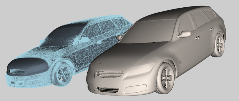
Figure 4 – Deformed geometry (left) with a wireframe overlay of original mesh highlighting change and original mesh (right)
Inference configuration. We trained a hierarchical machine learning model for a CFD flow field and drag predictions – we’ll explain that more soon. At runtime, we hosted these on different GPUs which allowed us to parallelize the inference of individual sub-models. To get inferences from the ML model, we specify the key inputs and parameters using inference configurations. These inputs include the decimated surface meshes of the car and a geometry for volume calculations. Additional input parameters include the batch size for inference, number of workers and other neural network associated hyperparameters.
Processed mesh. When a user requests an inference, the application generates a processed HDF5 file which contains the new mesh and the corresponding flow fields. These HDF5 files are then exposed to the end user via an interactive 3D visualization. There are some extra components that support the application: a function to convert meshes to HDF5 files, another function to apply the RBF to morph meshes based on user inputs, and finally a function to run inferences and gather outputs.
Deployment. Since this application is meant for demonstration purposes only, we designed it to run on a single compute instance, and chose a g5.12xlarge that includes 4 x GPUs that’s able to run the entire application. To speed the application, we distribute individual ML sub-models across the GPUs. To keep it all secure, we isolate the instances from the public internet in a private VPC. And we used NICE DCV to access the instance for an easier remote desktop experience.
Geometric and ML models
To enable engineers to rapidly iterate, potentially even during design conversations, our web application predicts the coefficient of drag (Cd) and the flow fields on unseen geometries. We used a hierarchy of ML models for the flow fields and drag predictions.
In both cases, we trained our models using synthetic data that we generated by morphing the open source DrivAer data set, and then ran full-fidelity CFD simulations on all these geometries using AWS Batch with the open-source TwinGraph framework.
Synthetic data generation. To create training data for this project, we used the RBF to strategically morph the underlying mesh of both the coupe and the SUV. This method has broad applicability and can be generically applied to many parametric and non-parametric STL meshes.
For each area of the car, we specified points in an overlayed 1000-point (10x10x10) cubic lattice, bounded by the dimensions of the car. This allowed us to create 400 variations (100 for each of the area of the car) that we used as the basis for ground-truth simulations. Figure 5 shows how we used the RBF to deform the mesh and create the training data for the ML model. Each time frame in the video corresponds to a different deformed mesh.
Figure 5 – Synthetic mesh generation using morphing of individual features of a car shown in sequence
After we created 400 variations of the base meshes, we used OpenFOAM to create CFD simulations with steady-state RANS simulations using the k-ω steady-state turbulence model with a fixed inlet velocity of 20m/s.
We ran these simulations in parallel using AWS Batch on c5.24xlarge instances using MPI for parallelism – this took around 7 hours to run. We could have chosen larger mesh sizes, but we settled on a mesh size that allowed resolving fine geometry – in a reasonable compute time.
Coefficient of drag with MeshGraphNets (MGN) – MGN is a deep-learning framework for learning mesh-based simulations which represents the mesh as a graph where information is propagated across the graph’s nodes and edges. MGN excels at efficiently capturing unstructured mesh topologies and it’s a great fit for predicting Cd values. To train the MGN model, we used the synthetic data that we generated using the RBF, and OpenFOAM. During training, we provided the underlying mesh and the Coefficient of Drag (Cd) metrics as inputs.
We then trained a model on 320 samples, with each mesh decimated while preserving topological features for computational efficiency, containing approximately 6,000 nodes. We used a p3.2xlarge instance for 500 epochs, with a total training time of 46 minutes.
The model achieved a MAPE (mean absolute percentage error) of 2.5% in drag coefficient (Cd) when predicting on unseen data, with an average inference time of 0.028 seconds per sample. Figure 6 shows the predicted vs. actual drag coefficient (Cd) plot for train, validation, and unseen test data (car meshes).
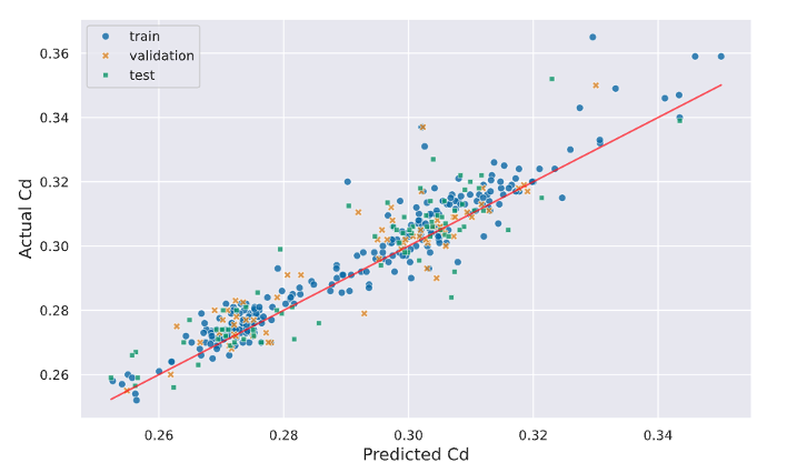
Figure 6: Predicted vs. actual drag coefficient (Cd) plot for train, validation, and unseen test data (i.e. car meshes).
Although the model didn’t match the ground truth CFD simulations exactly, this level of agreement from the MGN surrogate model may prove acceptable during the initial design iterations leading up to a final, high-fidelity simulation. After that comes real-world wind tunnel testing, which has an inherent uncertainty in measurements.
Flow Fields using deep convolutional neural networks (CNNs). To predict pressure distributions and velocity fields for full 3D flow, we used a CNN architecture called U-Net which has shown promise in high-resolution volume segmentation and regression tasks. This architecture included encoding and decoding convolutional layers with skip connections. We trained individual U-Nets for each of the pressure and velocity primary variables.
We converted the 3D volume outputs from 400 x OpenFOAM simulations into the training (375) and validation (25) ground-truth datasets. We used a p5.48xlarge instance with 8 x H100 GPUs for approximately 28 hours. We saw a volume RSME (root-mean-square-error) of around 3% for pressure, and 5% for combined velocity magnitudes, for unseen data not in the training or validation sets – although this is dependent on the degree of mesh warping away from the initial baseline mesh. Figure 7 shows the differences in velocity slices an unseen mesh.
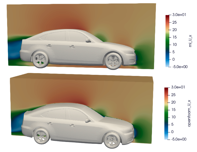
Figure 7: ML Predicted (Top) vs Ground Truth OpenFOAM (Bottom) X-Component Velocity
Business value creation
We’ve now shown how to rapidly build a minimally viable web interface that engineers can use to take advantage of these ML models to speed up the product engineering process. But now we need to couple this with a new business process so automakers can realize actual business value.
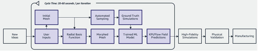
Figure 8: Overall product design iterations using machine learning surrogate models to accelerate the cycles
Using the speed of the ML surrogate models, it’s possible to explore hundreds of designs per week, and we can now make meetings more collaborative.
Instead of reviewing results from prior runs, engineers can solicit feedback from their peers real-time0, and get the results in 20-60 seconds, avoiding costly wait times. This will require engineers to think differently about product design reviews and meetings. Engineers will need to set expectations accordingly and be prepared to guide conversations. But this enables engineers to explore a greater design space than they otherwise could – especially given budget or time constraints. We’re confident this approach will lead to new innovations.
Conclusion
With the right combination of machine-learning and process change, automakers can use the architecture explained here to build tailored solutions to speed up the product engineering process, reduce the cost of compute, and explore a greater number of design options in a shorter period of time. If you or your team want to discuss the business case, a recommended implementation path with our Professional Services team, or technical solution blueprint in more detail, you can reach out to us at ask-hpc@amazon.com.