AWS Big Data Blog
Build an automatic data profiling and reporting solution with Amazon EMR, AWS Glue, and Amazon QuickSight
In typical analytics pipelines, one of the first tasks that you typically perform after importing data into your data lakes is data profiling and high-level data quality analysis to check the content of the datasets. In this way, you can enrich the basic metadata that contains information such as table and column names and their types.
The results of data profiling help you determine whether the datasets contain the expected information and how to use them downstream in your analytics pipeline. Moreover, you can use these results as one of the inputs to an optional data semantics analysis stage.
The great quantity and variety of data in modern data lakes make unstructured manual data profiling and data semantics analysis impractical and time-consuming. This post shows how to implement a process for the automatic creation of a data profiling repository, as an extension of AWS Glue Data Catalog metadata, and a reporting system that can help you in your analytics pipeline design process and by providing a reliable tool for further analysis.
This post describes in detail the application Data Profiler for AWS Glue Data Catalog and provides step-by-step instructions of an example implementation.
Overview and architecture
The following diagram illustrates the architecture of this solution.
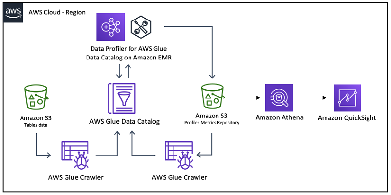
Data Profiler for AWS Glue Data Catalog is an Apache Spark Scala application that profiles all the tables defined in a database in the Data Catalog using the profiling capabilities of the Amazon Deequ library and saves the results in the Data Catalog and an Amazon S3 bucket in a partitioned Parquet format. You can use other analytics services such as Amazon Athena and Amazon QuickSight to query and visualize the data.
For more information about the Amazon Deequ data library, see Test data quality at scale with Deequ or the source code on the GitHub repo.
Metadata can be defined as data about data. Metadata for a table contains information like the table name and other attributes, column names and types, and the physical location of the files that contain the data. The Data Catalog is the metadata repository in AWS, and you can use it with other AWS services like Athena, Amazon EMR, and Amazon Redshift.
After you create or update the metadata for tables in a database (for example, adding new data to the table), either with an AWS Glue crawler or manually, you can run the application to profile each table. The results are stored as new versions of the tables’ metadata in the Data Catalog, which you can view interactively via the AWS Lake Formation console or query programmatically via the AWS CLI for AWS Glue.
For more information about the Data Profiler, see the GitHub repo.
The Deequ library does not support tables with nested data (such as JSON). If you want to run the application on a table with nested data, this must be un-nested/flattened or relationalized before profiling. For more information about useful transforms for this task, see AWS Glue Scala DynamicFrame APIs or AWS Glue PySpark Transforms Reference.
The following table shows the profiling metrics the application computes for column data types Text and Numeric. The computation of some profiling metrics for Text columns can be costly and is disabled by default. You can enable it by setting the compExp input parameter to true (see next section).
| Metric | Description | Data Type |
| ApproxCountDistinct | Approximate number of distinct values, computed with HyperLogLogPlusPlus sketches. |
Text / Numeric |
| Completeness | Fraction of non-null values in a column. | Text / Numeric |
| Distinctness | Fraction of distinct values of a column over the number of all values of a column. Distinct values occur at least one time. For example, [a, a, b] contains two distinct values a and b, so distinctness is 2/3. | Text / Numeric |
| MaxLength | Maximum length of the column. | Text |
| MinLength | Minimum length of the column. | Text |
| CountDistinct | Exact number of distinct values. | Text |
| Entropy | Entropy is a measure of the level of information contained in an event (value in a column) when considering all possible events (values in a column). It is measured in nats (natural units of information). Entropy is estimated using observed value counts as the negative sum of (value_count/total_count) * log(value_count/total_count). For example, [a, b, b, c, c] has three distinct values with counts [1, 2, 2]. Entropy is then (-1/5*log(1/5)-2/5*log(2/5)-2/5*log(2/5)) = 1.055. | Text |
| Histogram | The summary of values in a column of a table. Groups the given column’s values and calculates the number of rows with that specific value and the fraction of this value. | Text |
| UniqueValueRatio | Fraction of unique values over the number of all distinct values of a column. Unique values occur exactly one time; distinct values occur at least one time. Example: [a, a, b] contains one unique value b, and two distinct values a and b, so the unique value ratio is 1/2. | Text |
| Uniqueness | Fraction of unique values over the number of all values of a column. Unique values occur exactly one time. Example: [a, a, b] contains one unique value b, so uniqueness is 1/3. | Text |
| ApproxQuantiles | Approximate quantiles of a distribution. | Numeric |
| Maximum | Maximum value of the column. | Numeric |
| Mean | Mean value of the column. | Numeric |
| Minimum | Minimum value of the column. | Numeric |
| StandardDeviation | Standard deviation value of the column. | Numeric |
| Sum | Sum of the column. | Numeric |
Application description
You can run the application via spark-submit on a transient or permanent EMR cluster (see the “Creating an EMR cluster” section in this post for minimum version specification) with Spark installed and configured with the Data Catalog settings option Use for Spark table metadata enabled.
The following example code executes the application:
The following table summarizes the input parameters that the application accepts.
| Name | Type | Required | Default | Description |
--dbName (-d) |
String | Yes | N/A | Data Catalog database name. The database must be defined in the Catalog owned by the same account where the application is executed. |
--region (-r) |
String | Yes | N/A | AWS Region endpoint where the Data Catalog database is defined, for example us-west-1 or us-east-1. For more information, see Regional Endpoints. |
--compExp (-c) |
Boolean | No | false | If true, the application also executes “expensive” profiling analyzers on Text columns. These are CountDistinct, Entropy, Histogram, UniqueValueRatio, and Uniqueness. If false, only the following default analyzers are executed: ApproxCountDistinct, Completeness, Distinctness, MaxLength, MinLength. All analyzers for Numeric columns are always executed. |
--statsPrefix (-p) |
String | No | DQP | String prepended to the statistics names in the Data Catalog. The application also adds two underscores (__). This is useful to identify metrics calculated by the application. |
--s3BucketPrefix (-s) |
String | No | blank | Format must be s3Buckename/prefix. If specified, the application writes Parquet files with metrics in the prefixes db_name=…/table_name=…. |
--profileUnsupportedTypes (-u) |
Boolean | No | false | By default, the Amazon Deequ library only supports Text and Numeric columns. If this parameter is set to true, the application also profiles columns of type Boolean and Date. |
--noOfBins (-b) |
Integer | No | 10 | When --compExp (-c) is true, sets the number of maximum values to create for the Histogram analyzer for String columns. |
--quantiles (-q) |
Integer | No | 10 | Sets the number of quantiles to calculate for the ApproxQuantiles analyzer for numeric columns. |
Setting up your environment
The following walkthrough demonstrates how to create and populate a Data Catalog database with three tables, which simulates a process with monthly updates. For this post, you simulate three monthly runs: February 2, 2019, March 2, 2019, and April 2, 2019.
After table creation and after each monthly table update, you run the application to generate and update the profiling information for each table in the Data Catalog and Amazon S3 repository. The post also provides examples of how to query the data using the AWS CLI and Athena, and build a simple Amazon QuickSight dashboard.
This post uses the New York City Taxi and Limousine Commission (TLC) Trip Record Data on the Registry of Open Data on AWS. In particular, you use the tables yellow_tripdata, fhv_tripdata, and green_tripdata.
The following steps explain how to set up the environment.
Creating an EMR cluster
The first step is to create an EMR cluster. Connect to the cluster master node and execute the code via spark-submit. Make sure that the cluster version is at least 5.28.0 with at least Hadoop and Spark installed and that you use the Data Catalog as table metadata for Spark.

The master node should also be accessible via SSH. For instructions, see Connect to the Master Node Using SSH.
Downloading the application
You can download the source code and create a uber jar with all dependencies from the application GitHub repo. You can build the application as a uber jar with all dependencies using the Scala Build Tool (sbt) with the following commands (adjust the memory values according to your needs):
By default, the .jar file is created in the following path, relative to the project root directory:
./target/scala-2.11/data-profiler-for-aws-glue-data-catalog-assembly-1.0.jar
When the .jar file is available, copy it to the master node of the EMR cluster. One way to copy the file to the master node code is to copy it to Amazon S3 from the client where the file was created and download it from Amazon S3 to the master node.
For this post, copy the file in the /home/hadoop directory of the master node. The full path is /home/hadoop/data-profiler-for-aws-glue-data-catalog-assembly-1.0.jar.
Setting up S3 buckets and copy initial data
You use an S3 bucket to store the data that you profile. For this post, the bucket name is
s3://aws-big-data-blog-samples/
You need to create a bucket with a unique name in your account and store the data there. When the bucket is created and available, use the AWS CLI to copy the first set of files for January 2019 (therefore simulating the February 2, 2019, run) from the s3://nyc-tlc/ bucket. See the following code:
After you copy the data to your destination bucket, create a second bucket to store the files with the profiling metrics created by the application. This step is optional because you can write the metrics to a prefix in an existing bucket. See the following code:
You are now ready to create the database and tables metadata in the Data Catalog.
Creating metadata in the Data Catalog
The first step is to create a database in AWS Glue. You can create the database using the AWS CLI. See the following code:
Alternatively, on the AWS Glue console, choose Databases, Add database.

After you create the database, create a new AWS Glue Crawler to infer the schema of the data in the files you copied in the previous step. Complete the following steps:
- On the AWS Glue console, choose Crawler.
- Choose Add crawler.
- For Crawler name, enter
nyc-tlc-db-raw. - Choose Next.

- For Choose a data store, choose S3.
- For Crawl data in, choose Specified path in my account.
- For Include path, enter the S3 bucket and prefix where you copied the data earlier.
- Choose Next.

- In the Choose an IAM role section, select Choose an existing IAM role.
- Choose an IAM role that provides access to the S3 bucket and allows writing to the Data Catalog, or create a new one while creating this crawler.
- Choose Next.

- Choose the database you created earlier to store the tables’ metadata.
- Review the crawler properties and choose Finish.

You can run the crawler when it’s ready. It creates three new tables in the database. The following screenshot shows the update you receive that the crawler is complete.
- You can now use the Lake Formation console to check the tables are correct. See the following screenshot of the Tables.
 If you select one of the tables, the table version is now 0. See the following screenshot.
 You can also perform the same check using the AWS CLI. See the following code:
- Check the parameters in the table metadata to verify which values the crawler generated. See the following code:
- Check the metadata attributes for three columns in the same table. This post chooses the following columns because they have different data types, though any other column is suitable for this check. In the following code, the only attributes currently available for the columns are “
Name” and “Type:”
You can display the same information via the Lake Formation console. See the following screenshot.


You are now ready to execute the application.
First application execution
Connect to the EMR cluster master node via SSH and run the application with the following code (change the input parameters as needed, especially the value for the s3BucketPrefix parameter):
Profiling information in the metadata in the Data Catalog
When the application is complete, you can recheck the metadata via the Lake Formation console for the tables and verify that a new table version was created. See the following screenshot.

You can verify the same information via the AWS CLI. See the following code:
Check the metadata for the table and verify that the profiling information the application generated was successfully stored. In the following code, the parameter “DQP__Size” was generated, which contains the number of records in the table as calculated by the Deequ library:
Similarly, you can verify that the metadata for the columns you checked previously contains the profiling information the application generated. This is stored in the “Parameters” object for each column. Each new attribute starts with the string “DQP” as specified in the statsPrefix input parameter. See the following code:
The parameters named “DQP__name-x.x” are the results of the ApproxQuantiles Deequ analyzer for numeric columns; the number of quantiles is set via the –quantiles (-q) input parameter of the application. See the following code:
Profiling information in Amazon S3
You can now also verify that the profiling information was saved in Parquet format in the S3 bucket you specified in the s3BucketPrefix application input parameter. The following screenshot shows the buckets via the Amazon S3 console.

The data is stored using prefixes that are compatible with Apache Hive partitions. This is useful to optimize performance and costs when you use analytics services like Athena. The partitions are defined on db_name and table_name. The following screenshot shows the details of table_name=trip_data_yellow.

Each execution of the application generates one Parquet file appending data to the metrics table for each physical table.
Second execution after monthly table updates
To run the application after monthly table updates, complete the following steps:
- Copy the new files for February 2019 to simulate the March 2 monthly update of the system. See the following code:
- Run the
nyc-tlc-db-rawcrawler to update the table metadata to include the new files. The following screenshot shows that the three tables were updated successfully.
- Check that the crawler created a third version of the table. See the following code:
- Rerun the application to generate the new profiling metadata, entering the same code as before. To keep clean information, before storing new profiling information in the metadata, the application removes all custom attributes starting with the string specified in the “
statsPrefix” See the following code:Following a successful execution, a new version of the table was created. See the following code:
- Check the value of the
DQP__Sizeattribute; its value has changed. See the following code: - Check one of the columns you saw earlier to see the updated profiling properties values. See the following code:
Third execution after monthly tables updates
To run the application a third time, complete the following steps:
- Copy the new files for March 2019 to simulate the April 2 monthly update of the system. See the following code:
- Run the
nyc-tlc-db-rawcrawler to update the table metadata to include the new files. You now have five versions of the table metadata. See the following code: - Rerun the application to update the profiling information. See the following code:
- Check the
DQP__Sizeparameter to see its new updated value. See the following code: - Check one of the columns you saw earlier to the update profiling properties values. See the following code:
You can view and manage the same values via the Lake Formation console. See the following screenshot of the Edit column section.

Data profiling reporting with Athena and Amazon QuickSight
As demonstrated earlier, the application can save profiling information in Parquet format to an S3 bucket and prefix into db_name and table_name partitions. See the following code:
The application generates one Parquet file per execution.
Preparing metadata for profiler metrics data
To prepare the metadata for profiler metrics data, complete the following steps:
- On the Lake Formation console, create a new database with the name
deequprofilerdbto contain the metadata.
- On the AWS Glue console, create a new crawler with the name
deequ-profiler-metricsto infer the schema of the profiling information stored in Amazon S3.
The following screenshot shows the properties of the new crawler.

After you run the crawler, one table with the name deequ_profiler_metrics was created in the database. The table has the following columns.
| Name | Data Type | Partition | Description |
instance |
string | Column name the statistic in column “name” refers to. Set to “*” if entity is “Dataset”. |
|
entity |
string | Entity the statistic refers to. Valid values are “Column” and “Dataset”. |
|
name |
string | Metrics name, derived from the Deequ Analyzer used for the calculation. | |
value |
double | Value of the metric. | |
type |
string | Data type of the column if entity is “Column”, blank otherwise. |
|
db_name_embed |
string | Database name, same values as in partition “db_name”. |
|
table_name_embed |
string | Table name, same values as in partition “table_name”. |
|
profiler_run_dt |
date | Date the profiler application was run. | |
profiler_run_ts |
timestamp | Date/time the profile application was run; it can also be used as execution identifier. | |
db_name |
string | 1 | Database name. |
table_name |
string | 2 | Table name. |
Reporting with Athena
You can use Athena to run a query that checks the statistics for a column in the database for the execution you ran in March 2019. See the following code:
The following screenshot shows the query results.

Reporting with Amazon QuickSight
To create a dashboard in Amazon QuickSight based on the profiling metrics data the application generated, complete the following steps:
- Create a new QuickSight dataset called
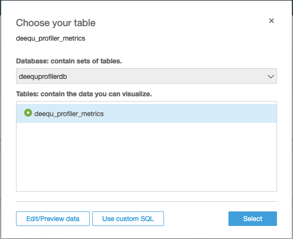
deequ_profiler_metricswith Athena as the data source.
- In the Choose your table section, select the profiling metrics table that you created earlier.
- Import the data into SPICE.

After you create the dataset, you can view it and edit its properties. For this post, leave the properties unchanged.

You are now ready to build visualizations and dashboards.
The following images in this section show a simple analysis with controls that allow for the selection of the Database, Table profiled, Entity, Column, and Profiling Metric.
| Control Name | Mapped Column |
| Database | db_name |
| Table | table_name |
| Entity | entity |
| Column | instance |
| Profiling Metric | name |
For more information about adding controls, see Create Amazon QuickSight dashboards that have impact with parameters, on-screen controls, and URL actions.
For example, you can select the Size metric of a specific table to see how many records are available in the table after each monthly load. See the following screenshot.

Similarly, you can use the same analysis to see how a specific metric changes over time for a column. The following screenshot shows that the mean of the fare_amount column changes after each monthly load.

You can select any metric calculated on any column, which makes for a very flexible profiling data reporting system.

Conclusion
This post demonstrated how to extend the metadata contained in the Data Catalog with profiling information calculated with an Apache Spark application based on the Amazon Deequ library running on an EMR cluster.
You can query the Data Catalog using the AWS CLI. You can also build a reporting system with Athena and Amazon QuickSight to query and visualize the data stored in Amazon S3.
Special thanks go to Sebastian Schelter at Amazon Search and Sven Hansen and Vincent Gromakowski at AWS for their help and support
About the Author
 Francesco Marelli is a senior solutions architect at Amazon Web Services. He has lived and worked in London for 10 years, after that he has worked in Italy, Switzerland and other countries in EMEA. He is specialized in the design and implementation of Analytics, Data Management and Big Data systems, mainly for Enterprise and FSI customers. Francesco also has a strong experience in systems integration and design and implementation of web applications. He loves sharing his professional knowledge, collecting vinyl records and playing bass.