AWS Compute Blog
Optimizing EC2 Workloads with Amazon CloudWatch
This post is written by David (Dudu) Twizer, Principal Solutions Architect, and Andy Ward, Senior AWS Solutions Architect – Microsoft Tech.
In December 2020, AWS announced the availability of gp3, the next-generation General Purpose SSD volumes for Amazon Elastic Block Store (Amazon EBS), which allow customers to provision performance independent of storage capacity and provide up to a 20% lower price-point per GB than existing volumes.
This new release provides an excellent opportunity to right-size your storage layer by leveraging AWS’ built-in monitoring capabilities. This is especially important with SQL workloads as there are many instance types and storage configurations you can select for your SQL Server on AWS.
Many customers ask for our advice on choosing the ‘best’ or the ‘right’ storage and instance configuration, but there is no one solution that fits all circumstances. This blog post covers the critical techniques to right-size your workloads. We focus on right-sizing a SQL Server as our example workload, but the techniques we will demonstrate apply equally to any Amazon EC2 instance running any operating system or workload.
We create and use an Amazon CloudWatch dashboard to highlight any limits and bottlenecks within our example instance. Using our dashboard, we can ensure that we are using the right instance type and size, and the right storage volume configuration. The dimensions we look into are EC2 Network throughput, Amazon EBS throughput and IOPS, and the relationship between instance size and Amazon EBS performance.
The Dashboard
It can be challenging to locate every relevant resource limit and configure appropriate monitoring. To simplify this task, we wrote a simple Python script that creates a CloudWatch Dashboard with the relevant metrics pre-selected.
The script takes an instance-id list as input, and it creates a dashboard with all of the relevant metrics. The script also creates horizontal annotations on each graph to indicate the maximums for the configured metric. For example, for an Amazon EBS IOPS metric, the annotation shows the Maximum IOPS. This helps us identify bottlenecks.
Please take a moment now to run the script using either of the following methods described. Then, we run through the created dashboard and each widget, and guide you through the optimization steps that will allow you to increase performance and decrease cost for your workload.
Creating the Dashboard with CloudShell
First, we log in to the AWS Management Console and load AWS CloudShell.

Once we have logged in to CloudShell, we must set up our environment using the following command:
The commands preceding download the script and configure the CloudShell environment with the correct Python settings to run our script. Run the following command to create the CloudWatch Dashboard.
At its most basic, you just must specify the list of instances you are interested in (i-example1 and i-example2 in the preceding example), and the Region within which those instances are running (eu-west1 in the preceding example). For detailed usage instructions see the README file here. A link to the CloudWatch Dashboard is provided in the output from the command.
Creating the Dashboard Directly from your Local Machine
If you’re familiar with running the AWS CLI locally, and have Python and the other pre-requisites installed, then you can run the same commands as in the preceding CloudShell example, but from your local environment. For detailed usage instructions see the README file here. If you run into any issues, we recommend running the script from CloudShell as described prior.
Examining Our Metrics
Once the script has run, navigate to the CloudWatch Dashboard that has been created. A direct link to the CloudWatch Dashboard is provided as an output of the script. Alternatively, you can navigate to CloudWatch within the AWS Management Console, and select the Dashboards menu item to access the newly created CloudWatch Dashboard.
The Network Layer
The first widget of the CloudWatch Dashboard is the EC2 Network throughput:
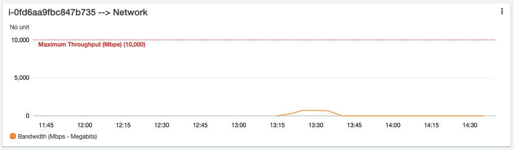
The automatic annotation creates a red line that indicates the maximum throughput your Instance can provide in Mbps (Megabits per second). This metric is important when running workloads with high network throughput requirements. For our SQL Server example, this has additional relevance when considering adding replica Instances for SQL Server, which place an additional burden on the Instance’s network.
In general, if your Instance is frequently reaching 80% of this maximum, you should consider choosing an Instance with greater network throughput. For our SQL example, we could consider changing our architecture to minimize network usage. For example, if we were using an “Always On Availability Group” spread across multiple Availability Zones and/or Regions, then we could consider using an “Always On Distributed Availability Group” to reduce the amount of replication traffic. Before making a change of this nature, take some time to consider any SQL licensing implications.
If your Instance generally doesn’t pass 10% network utilization, the metric is indicating that networking is not a bottleneck. For SQL, if you have low network utilization coupled with high Amazon EBS throughput utilization, you should consider optimizing the Instance’s storage usage by offloading some Amazon EBS usage onto networking – for example by implementing SQL as a Failover Cluster Instance with shared storage on Amazon FSx for Windows File Server, or by moving SQL backup storage on to Amazon FSx.
The Storage Layer
The second widget of the CloudWatch Dashboard is the overall EC2 to Amazon EBS throughput, which means the sum of all the attached EBS volumes’ throughput.
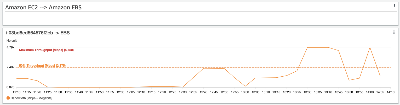
Each Instance type and size has a different Amazon EBS Throughput, and the script automatically annotates the graph based on the specs of your instance. You might notice that this metric is heavily utilized when analyzing SQL workloads, which are usually considered to be storage-heavy workloads.
If you find data points that reach the maximum, such as in the preceding screenshot, this indicates that your workload has a bottleneck in the storage layer. Let’s see if we can find the EBS volume that is using all this throughput in our next series of widgets, which focus on individual EBS volumes.
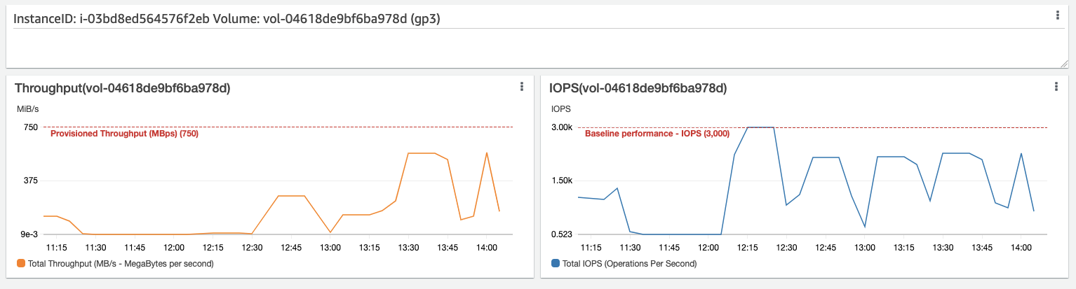
And here is the culprit. From the widget, we can see the volume ID and type, and the performance maximum for this volume. Each graph represents one of the two dimensions of the EBS volume: throughput and IOPS. The automatic annotation gives you visibility into the limits of the specific volume in use. In this case, we are using a gp3 volume, configured with a 750-MBps throughput maximum and 3000 IOPS.
Looking at the widget, we can see that the throughput reaches certain peaks, but they are less than the configured maximum. Considering the preceding screenshot, which shows that the overall instance Amazon EBS throughput is reaching maximum, we can conclude that the gp3 volume here is unable to reach its maximum performance. This is because the Instance we are using does not have sufficient overall throughput.
Let’s change the Instance size so that we can see if that fixes our issue. When changing Instance or volume types and sizes, remember to re-run the dashboard creation script to update the thresholds. We recommend using the same script parameters, as re-running the script with the same parameters overwrites the initial dashboard and updates the threshold annotations – the metrics data will be preserved. Running the script with a different dashboard name parameter creates a new dashboard and leaves the original dashboard in place. However, the thresholds in the original dashboard won’t be updated, which can lead to confusion.
Here is the widget for our EBS volume after we increased the size of the Instance:

We can see that the EBS volume is now able to reach its configured maximums without issue. Let’s look at the overall Amazon EBS throughput for our larger Instance as well:

We can see that the Instance now has sufficient Amazon EBS throughput to support our gp3 volume’s configured performance, and we have some headroom.
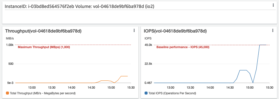
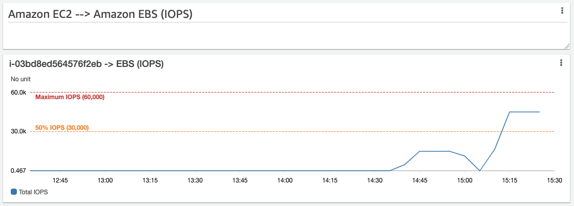
Now, let’s swap our Instance back to its original size, and swap our gp3 volume for a Provisioned IOPS io2 volume with 45,000 IOPS, and re-run our script to update the dashboard. Running an IOPS intensive task on the volume results in the following:

As you can see, despite having 45,000 IOPS configured, it seems to be capping at about 15,000 IOPS. Looking at the instance level statistics, we can see the answer:

Much like with our throughput testing earlier, we can see that our io2 volume performance is being restricted by the Instance size. Let’s increase the size of our Instance again, and see how the volume performs when the Instance has been correctly sized to support it:
We are now reaching the configured limits of our io2 volume, which is exactly what we wanted and expected to see. The instance level IOPS limit is no longer restricting the performance of the io2 volume:
Using the preceding steps, we can identify where storage bottlenecks are, and we can identify if we are using the right type of EBS volume for the workload. In our examples, we sought bottlenecks and scaled upwards to resolve them. This process should be used to identify where resources have been over-provisioned and under-provisioned.
If we see a volume that never reaches the maximums that it has been configured for, and that is not subject to any other bottlenecks, we usually conclude that the volume in question can be right-sized to a more appropriate volume that costs less, and better fits the workload.
We can, for example, change an Amazon EBS gp2 volume to an EBS gp3 volume with the correct IOPS and throughput. EBS gp3 provides up to 1000-MBps throughput per volume and costs $0.08/GB (versus $0.10/GB for gp2). Additionally, unlike with gp2, gp3 volumes allow you to specify provisioned IOPS independently of size and throughput. By using the process described above, we could identify that a gp2, io1, or io2 volume could be swapped out with a more cost-effective gp3 volume.
If during our analysis we observe an SSD-based volume with relatively high throughput usage, but low IOPS usage, we should investigate further. A lower-cost HDD-based volume, such as an st1 or sc1 volume, might be more cost-effective while maintaining the required level of performance. Amazon EBS st1 volumes provide up to 500 MBps throughput and cost $0.045 per GB-month, and are often an ideal volume-type to use for SQL backups, for example.
Additional storage optimization you can implement
Move the TempDB to Instance Store NVMe storage – The data on an SSD instance store volume persists only for the life of its associated instance. This is perfect for TempDB storage, as when the instance stops and starts, SQL Server saves the data to an EBS volume. Placing the TempDB on the local instance store frees the associated Amazon EBS throughput while providing better performance as it is locally attached to the instance.
Consider Amazon FSx for Windows File Server as a shared storage solution – As described here, Amazon FSx can be used to store a SQL database on a shared location, enabling the use of a SQL Server Failover Cluster Instance.
The Compute Layer
After you finish optimizing your storage layer, wait a few days and re-examine the metrics for both Amazon EBS and networking. Use these metrics in conjunction with CPU metrics and Memory metrics to select the right Instance type to meet your workload requirements.
AWS offers nearly 400 instance types in different sizes. From a SQL perspective, it’s essential to choose instances with high single-thread performance, such as the z1d instance, due to SQL’s license-per-core model. z1d instances also provide instance store storage for the TempDB.
You might also want to check out the AWS Compute Optimizer, which helps you by automatically recommending instance types by using machine learning to analyze historical utilization metrics. More details can be found here.
We strongly advise you to thoroughly test your applications after making any configuration changes.
Conclusion
This blog post covers some simple and useful techniques to gain visibility into important instance metrics, and provides a script that greatly simplifies the process. Any workload running on EC2 can benefit from these techniques. We have found them especially effective at identifying actionable optimizations for SQL Servers, where small changes can have beneficial cost, licensing and performance implications.