Deploying a Level 3 Digital Twin Virtual Sensor with Ansys on AWS

This post was contributed by Ross Pivovar and Adam Rasheed from AWS, and Matt Adams from Ansys

A common Digital Twin use case we hear from our customers is the need for virtual sensors where physical sensors are replaced with a prediction model. Virtual sensors work well when measuring a property is difficult, expensive, or impractical. In a previous post, we described a Digital Twin leveling index to help customers understand their use cases and the technologies required to achieve their goals. A level 3 (L3) Digital Twin focuses on predicting unmeasured quantities using Internet of Things (IoT) data.

Virtual sensors are often based on either machine learning (ML) or physics-based models. ML models require large training sets to cover the full domain of possible outcomes and have potential safety concerns with predicting an outcome. Comparatively, physics-based models only require small validation sets to confirm accuracy. However, these models do not reflect environmental changes, such as degrading equipment or changing assumptions used to develop the initial model.

In this post, we’ll describe how to build and deploy an L3 Digital Twin virtual sensor using an Ansys model on AWS. Ansys provides a variety of finite element method (FEM) and computational fluid dynamics (CFD) simulation applications, which are critical to developing a digital twin. We’ll use the Ansys Twin Builder and Twin Deployer to build the model and then AWS IoT TwinMaker and the AWS TwinFlow framework to simplify building, deploying, and orchestrating predictive models at scale on AWS.

Building the Digital Twin

For our use case, an energy company is increasing the fleet size of their natural gas (NG) compressor trains. A compressor train uses a sequential series of compressors to incrementally compress a gas into a liquid for compact storage in pressurized containers or long-distance transport. The energy company decided to significantly decrease setup and maintenance costs by converting the discharge pressures sensors in their NG compressor trains from physical to virtual. A compressor digital twin provides the virtual sensors.

For this proof of concept, we used a Modelica system model with Ansys Twin Builder to develop a thermodynamic model of the compressor, which we deployed on AWS using Ansys Twin Deployer. Ansys Twin Builder is an open solution that allows engineers to create simulation-based digital twins and validate the accuracy of their digital twin models. Ansys Twin Deployer is used to execute Ansys Twin Builder models with a scalable independent licensing structure which does not require Ansys Twin Builder or other Ansys licenses to run. Ansys Twin Builder can also be used to convert the high-fidelity model into a reduced order model (ROM) for short runtime physics based digital twin prediction of a single stage compressor, shown in Figure 1.

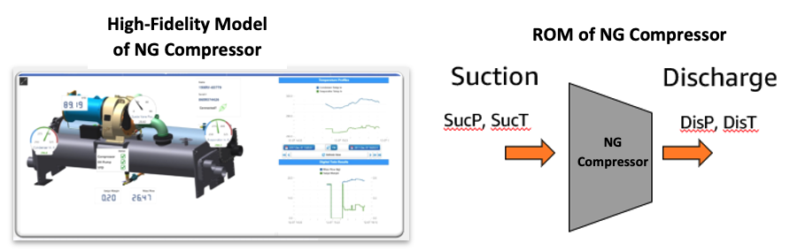
Figure 1 Ansys Twin Builder converts high-fidelity to Reduced Order Model (ROM).

To simulate a multi-stage compressor train, we replicated the Ansys model for a single stage (n times for n stages) and arranged them so that the results of each stage are fed into the subsequent downstream stage, like in Figure 2.

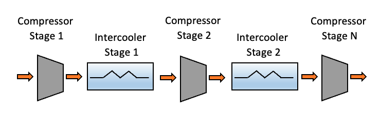
Figure 2 Output of upstream compressor stages serve as inputs to downstream stages.

We used a two-stage compressor train in this post. Between each compressor stage is an intercooler to decrease fluid temperature, which decreases the required thermodynamic work of the subsequent compressor. Since the inputs of each subsequent stage rely on a combination of physical sensor and virtual sensor predictions, there is an inherent increase in uncertainty for each stage. The energy company needs to have at least one NG compressor train with a full set of physical sensors to compare and calibrate predictions.

An operator may be concerned with over pressurization and uncertainty propagation in each stage. A constant bias value could be added to the measured sensor data, but a constant value does not change with system inputs or compressor stages. This is not a preferred approach since a constant bias that does not adapt to the environment will need to be quite large to cover all possibilities.

To eliminate this issue, we used an ML model trained on the IoT inputs and physics predictions (Ansys output) to adaptively bias the physics predictions. The conservative values have a low probability of the true pressure being above the prediction. We trained an ML corrector model to predict the residuals where the bias is adjusted based on the physics prediction and the stage of the compressor train. The residuals are defined as the difference between the true measured calibration data and the physics prediction.

The chosen ML model uses a quantile loss function and predicts the 95^th percentile of the physics residuals. Any percentile can be chosen, but the 95^th is a typical value used by regulators to ensure conservatism. This prediction then serves as a conservative bias for the physics prediction.

The combination of physics and ML-corrector model can be labeled as a “predictor/corrector” model. Figure 3 shows the effect of the predictor/corrector model.

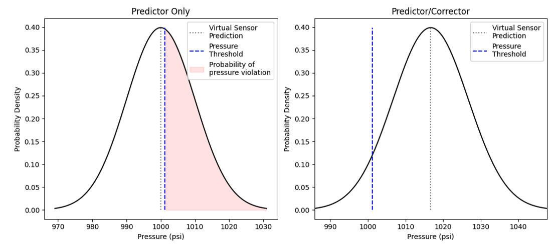
Figure 3 Probability effects of quantile ML model shifts.

A normal distribution shown in the left plot demonstrates the best estimate without bias. The plot shows the virtual sensor output (grey dotted lined) and the uncertainty associated with this prediction (black solid line). If the compressor train pressure prediction is close but not greater than the safety pressure threshold, there is nearly a 50% probability (shaded region) that the true pressure of the system violated the pressure threshold and the operator is unaware. The right plot displays physics prediction with the addition of a bias and tells the operator the pressure threshold was violated.

Validating the Predictor/Corrector Model

Prior to deploying the virtual sensors, we validated the predictor/corrector model to check that it was working as expected. We also improved performance by preprocessing the raw data with a Kalman filter (KF) to remove excess sensor noise, as shown in Figure 4.

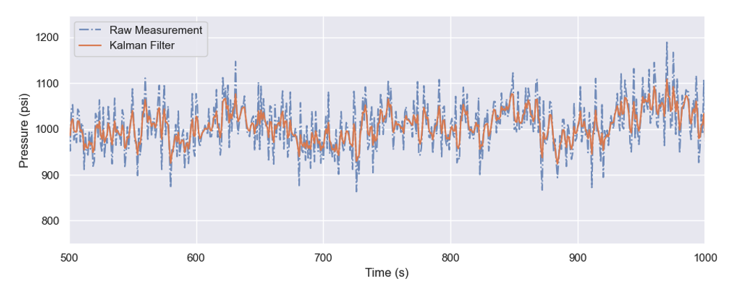
Figure 4 Demonstration of sensor noise reduction by utilizing an Kalman Filter.

We reduced the raw data (dashed blue line) sensor noise with a Kalman Filter (solid orange line). In our example, we uses the filtered data going forward. Because data filtering is a common task for sensor data, the KF functionality is provided in the AWS TwinFlow framework. Using the KF-filtered data, we now compare physical sensor measurements with the virtual sensor predictions in more detail in Figure 5.

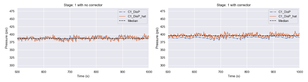
Figure 5 Comparison of predictor and predictor/corrector output pressure for stage 1 of a compressor train

The left plot in Figure 5 displays the physical sensor measurement for compressor discharge pressure “C1_DisP” (blue line) and the predictor only estimate “C1_DisP_hat” (orange line) for the first stage. We observe a median underprediction bias of -2.5psi (-0.6%) indicating the uncorrected physics model is sufficiently predicting the outlet pressure for the first stage. The right plot in Figure 5 displays the predictor/corrector results with a median bias of 6.6psi (1.7%) showing that the prediction is conservative.

Although the uncorrected physics prediction more closely reflects the actual sensor measurement for the first stage, this becomes an issue in the second and subsequent compressor stages. In Figure 6, we observe the predictions for the second stage.

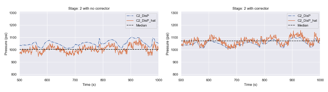
Figure 6 Comparison of predictor and predictor/corrector output pressure for stage 2 of a compressor train

The uncorrected physics predictions in the left plot are underpredicting the measured discharge pressure by a median -44.2psi (-4.2%). This is undesirable because the virtual sensor is not catching an over-pressure situation. For a compressor train with many stages, the physics model will appreciably deviate even further from reality due to the uncertainty propagation. The right plot of Figure 6 demonstrates the predictor/corrector model safely shifts the result to a conservative median bias of 24.2psi (2.3%).

In our example, we want a virtual sensor that’s conservative (relative to the real sensor measurement) to avoid over-pressure situations. Other use cases might want the virtual sensor to over-predict the real sensor measurement or be as close as possible to the real sensor measurement. We set the bias amount (or zero-bias) in the corrector model.

Virtual Sensor Workflow and Architecture

We used the AWS TwinFlow framework to build, deploy, and orchestrate predictive models at scale across a distributed computing architecture. The framework also probabilistically updates model parameters using real-world data and calculates prediction uncertainty while maintaining a fully auditable history. The TwinFlow framework is in development and we will release it as open-source in Q3 this year. Our overall workflow is in Figure 7.

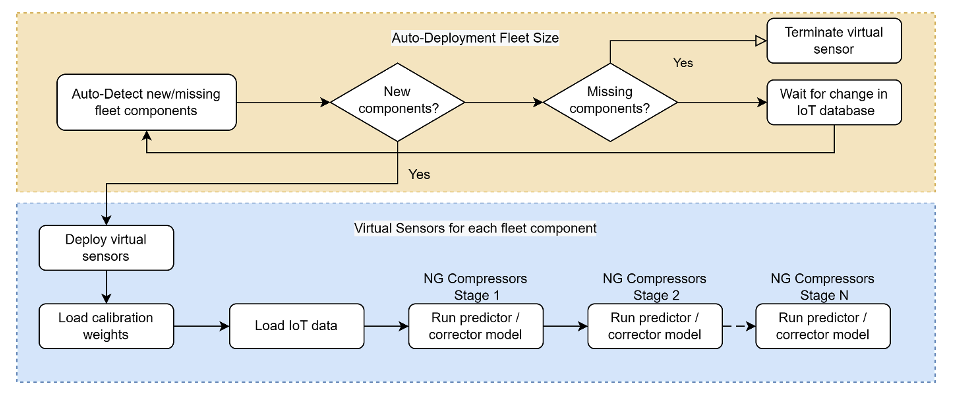
Figure 7 TwinFlow workflow enabling level 3 digital twin.

The top half describes the auto-deployment of virtual sensors, and the bottom half is the workflow of a virtual sensor. The auto-deployment branch will periodically check Amazon Simple Queue Service (Amazon SQS) for new component Amazon Simple Storage Service (Amazon S3) events and automatically create or destroy virtual sensors. Auto-deployment provides cloud elasticity saving time for virtual sensor setup and money by automatically scaling down idle infrastructure.

A deployed virtual sensor will first load the corrector calibration weights stored in an Amazon S3 bucket. Next, we stream the IoT data from a data source like Amazon Timestream and the virtual sensor makes predictions at a user-specified frequency for the discharge pressures throughout the compressor train. You can see our architecture for supporting this workflow in Figure 8.

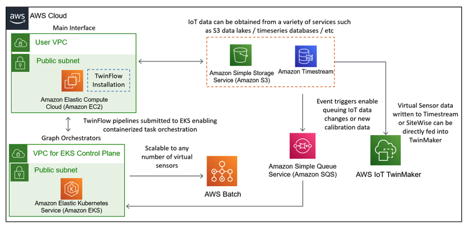
Figure 8 AWS architecture for virtual sensors.

TwinFlow orchestrates the required workflow tasks. We deployed the virtual sensors from the Amazon Elastic Compute Cloud (Amazon EC2) instance where TwinFlow was installed. TwinFlow uses a graph orchestrator on an Amazon Elastic Kubernetes Service (Amazon EKS) control plane to manage complex asynchronous execution of tasks. We used a Python TwinFlow pipeline file to define tasks, relationships, and configuration, like virtual sensor sampling frequency.

We deployed each virtual sensor on AWS Batch to enable deployment at scale, where each virtual sensor is accessing necessary input data from data sources like Amazon S3 and Amazon Timestream. Metadata in the Amazon S3 data lake informs the individual virtual sensors which IoT data streams to ingest. S3 Event triggers, like new or missing sensors, notify an Amazon SQS queue where the Amazon EKS cluster monitors the queue and deploys or terminates virtual sensors based on Amazon S3 data.

Once the virtual sensors are deployed, their output can be directed for further processing. A single compressor train may have dozens or hundreds of IoT output, physical or virtual. You can visualize the sensor data – both physical and virtual – with AWS TwinMaker on an L2 spatial digital twin in real time. The virtual sensor output can also be directed to downstream services for further analysis, like anomaly detection in Amazon Lookout for Equipment or custom ML/analytics in Amazon SageMaker.

Summary

In this post, we showed how you can build a virtual sensor on AWS using L3 digital twins. In future posts, we’ll discuss converting an L3 virtual sensor to a self-calibrating virtual sensor to enable adaptation to changing environments.

Our next post will also discuss methods for determining when you need new calibration data to ensure peak accuracy of the virtual sensor.

If you want to request a proof of concept or if you have feedback on the AWS tools, please reach out to us at ask-hpc@amazon.com.