Streamlining distributed ML workflow orchestration using Covalent with AWS Batch

This post was contributed by Ara Ghukasyan, Research Software Engineer, and Santosh Kumar Radha, Head of R&D and Product, and William Cunningham, Head of HPC at Agnostiq, with Perminder Singh, Worldwide Partner Solution Architect, Tejas Rakshe, Sr. Global Alliance Manager at AWS.

Complicated multi-step workflows can be challenging to deploy, especially when using a variety of high-compute resources. Consider machine learning workflows which often involve computationally intensive preprocessing, training, and characterization steps that could require specialized hardware. Experiments of this nature fall into the broad category of heterogeneous computing. For instance, it’s common in machine learning to use GPUs for training neural networks, while also using CPUs to handle lighter tasks. Moreover, if the model also has non-learnable hyperparameters, then multiple repetitions of the experiment will be necessary to fine-tune to their values. This leads to massive workloads that require cloud resources in practical applications.

To address this common challenge, many practitioners opt to explore the hyperparameter space through concurrent runs, deploying parallel instances to handle each combination of parameters. Beyond this, however, coordinating an efficient and reproducible experiment can require time and cloud expertise that many users do not have.

Covalent is an open-source orchestration tool that streamlines the deployment of distributed workloads on AWS resources. It provides powerful abstractions that elevate the user-resource interaction, especially in the context of high-compute experiments. Covalent eliminates overhead by parsing workflows to orchestrate their sub-tasks using a serverless HPC architecture. This means that users can easily expand their computing capacity by recruiting cloud resources whenever demand spikes—a concept known as “cloud bursting”.

Covalent is suitable for a wide range of users, including machine learning practitioners, data scientists, and anyone interested in a Pythonic tool for running heterogenous computations from their local environment.

In what follows, we use a sample problem to outline key concepts in Covalent and develop a machine learning workflow for AWS Batch in just a handful of steps. To conclude, we showcase some material benefits of using Covalent, as reflected in saved compute-hours and shorter wall times.

Resources

Covalent can interact with many compute resources—including several AWS resources—using an interface based on modular executor plugins. In this example, we use AWS Batch, which provides managed environments for provisioning a broad variety of instances in the Amazon Elastic Compute Cloud (Amazon EC2). A cluster of Amazon EC2 P3 instances is a good choice for leveraging GPU acceleration to train and validate our machine learning model. An Amazon Simple Storage Service (Amazon S3) bucket will serve our data storage needs in this example.

We will use Covalent’s AWS Batch Executor to interact with all these resources.

Sample Problem

Let’s consider the problem of training a neural network for object recognition in a supervised setting. Specifically, we adapt the code available publicly here. The goal is to identify abnormal brain tissue in magnetic resonance images (MRI), given matching “segmentation masks” that indicate the desired solution.

In the Figure 1, Input image on the left is an MRI slice of a human head. Input image on the right shows a lesion highlighted in upper right. The segmentation mask on the right uses pixels 0 or 1 to mark the lesion shape and location.

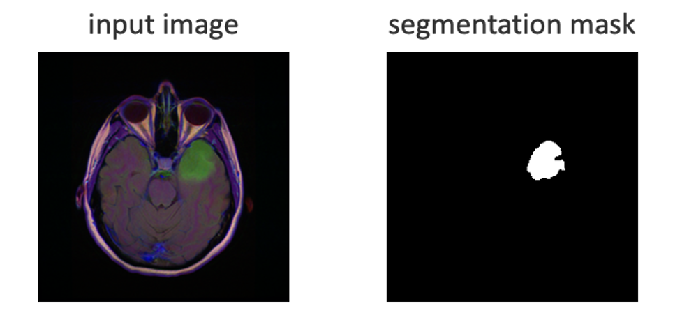
Figure 1 – Input datum represented by an enhanced MRI image and matching mask of the lesion area.

In this problem we have (aside from the learnable parameters): the number of training epochs, the learning rate, and the target size for image reduction (in preprocessing) as some additional hyperparameters. For clarity going forward, we employ a simple dataclass as a container for these values:

@dataclass(frozen=True)
class HyperParams:
    batch_size: int
    epochs: int
    learning_rate: float
    image_size: int

Let’s proceed with designing a workflow to carry out the experiment.

Basic Workflow Design

Perhaps the most straightforward way to explore the hyperparameter space is to use a for loop over an arbitrary subset of points. This is implemented in hp_sweep(), below:

def hp_sweep(data_dir: Path, params_list: List[HyperParams], transform: Callable):
    training_results = {}
    for i, ps in enumerate(params_list):
        input_paths = preprocess_images(data_dir, ps.image_size, transform)
        training_result = train_neural_network(input_paths, ps, label=i + 1)
        output_dir = write_predictions(training_result)
        download_output(output_dir)

        training_result[ps] = training_result

    return training_results

This is what happens inside the above function: For each point ps, the inputs are processed and shrunk to ps.image_size by ps.image_size pixels in preprocess_images(). Next, the training/validation loop runs for ps.epochs -many epochs inside train_neural_network(), using ps.learning_rate for the optimizer backend. Eventually, the trained model state is saved, and its location is returned inside the training_result object. Passing this to write_predictions() loads the trained model and tests it against new, unseen inputs. Finally, download_output() downloads outputs from a remote location.

Obviously, the workflow iterates through hyperparameter space one point at a time. While brief and readable, this is hardly optimal. Using Covalent can significantly improve this workflow by introducing parallelism and efficiently distributing individual tasks. As we’ll show in the next section, this requires little more than adding a handful of decorators.

Introduction to Covalent

Covalent is an open-source workflow orchestration tool designed for running distributed experiments over HPC clusters, quantum computers, GPU arrays, and cloud services like AWS Batch.

Architecture

Covalent utilizes a serverless HPC architecture that provisions resources on-demand to guarantee scalable, cost-effective deployments that avoid any idle time across distributed tasks. Users dispatch workflows from their local environment with the Covalent SDK. Workflow tasks are then managed by Covalent, which executes them asynchronously, in arbitrary environments and on arbitrary backends. Each task can be customized in this way to seamlessly integrate computations across inter-dependent tasks on heterogenous hardware.

The diagram below illustrates these interactions as they pertain to the present example and beyond. With Covalent, we can easily use several different AWS resources for the sub-tasks comprising a given workflow. For this tutorial, it’s enough to rely solely on AWS Batch.

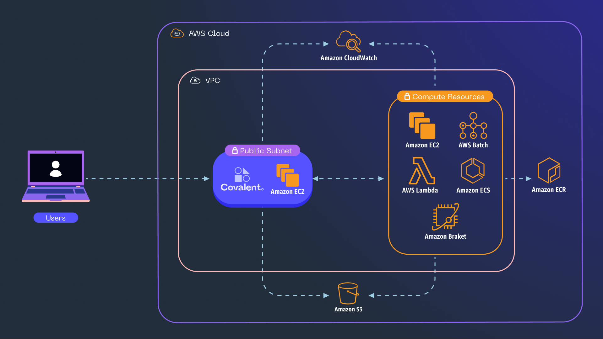
Figure 2 – An architecture diagram depicting a remote instance of Covalent that receives user-dispatched workflows and orchestrates them on AWS resources.

Covalent architecture diagram. User interacts with Covalent. Covalent interacts with AWS resources.

Developing with Covalent

The Covalent SDK provides a Pythonic interface that uses three main elements: the electron decorator, executor objects, and the lattice decorator. These elements help users to define complex workflows in a lightweight and non-destructive manner, with only minor changes to their experimental code. Let’s briefly review the electron, executor, and lattice constructs to better understand their purpose.

Electrons (Tasks)

The electron decorator (@ct.electron) is used to convert a function into a remotely-executable task that Covalent can deploy to an arbitrary resource. Users specify resources and constraints for each electron by passing various executor objects to electron decorators.

Executors

Executor objects play a key role in Covalent by containerizing task execution. They enable the deployment to scale along with the workflow function and tasks to be executed in a serverless manner. For the user, an executor codifies the execution parameters while abstracting away the execution process. Executors are resource-specific and a variety of Covalent executor plugins are supported for this purpose.

Below, we use Covalent’s AWSBatchExecutor to access P3 Amazon EC2 instances in our AWS Batch compute environment. Since the instance type is inferred from the executor’s parameters, we set num_gpus=1 to target P3 instances specifically. We then use the electron decorator to create electrons from each function that implements a step in our workflow. Finally, awsbatch_exec is passed to @ct.electron for any function that we wish to execute on an instance:

import covalent as ct

# create an executor to pass to electrons below
awsbatch_exec = ct.executor.AWSBatchExecutor(
    credentials="~/.aws/credentials",
    s3_bucket_name="my-s3-bucket",
    batch_queue="my-batch-queue",
    batch_job_log_group_name="my-log-group",
    time_limit=7200,
    vcpu=2,
    memory=4,
    num_gpus=1,
)

# use `@ct.electron` to make electrons from individual tasks

@ct.electron(executor=awsbatch_exec)
def preprocess_images(data_dir, image_size, transform=None):
    """function that performs image preprocessing"""
    ...

@ct.electron(executor=awsbatch_exec)
def train_neural_network(input_paths, params, label):
    """function that runs the training/validation loop"""
    ...

@ct.electron(executor=awsbatch_exec)
def write_predictions(training_result):
    """function that tests the model against unseen data"""
    ...

@ct.electron(executor="local")  # execute in local process pool
def download_output(output_dir):
    """function that downloads prediction outputs from S3 bucket"""
    ...

The Lattice (Workflow)

The lattice decorator (@ct.lattice) converts a function composed of electrons into a manageable workflow. It does this by wrapping the function in a callable Lattice object. We create the lattice for our hyperparameter sweep by simply adding this decorator on top of hp_sweep():

# use `@ct.lattice` to make the "lattice" from a function that calls electrons

@ct.lattice
def hp_sweep(data_dir: Path, params_list: List[HyperParams], transform: Callable):
    training_results = {}
    for i, ps in enumerate(params_list):
        input_paths = preprocess_images(data_dir, ps.image_size, transform)
        training_result = train_neural_network(input_paths, ps, label=i + 1)
        output_dir = write_predictions(training_result)
        download_output(output_dir)

        training_result[ps] = training_result

    return training_results

How to Dispatch Workflows

A convenient feature is that the @ct.electron and @ct.lattice decorators have practically no effect on underlying code, unless the lattice is dispatched using ct.dispatch(). When electron-decorated functions are called in any other context, they run and return as usual, with minimal additional overhead. This lets users preserve core functionality while introducing Covalent to existing code or developing from scratch with the Covalent SDK. The resulting code also remains testable, which is another important benefit of this non-destructive design.

# dispatch workflow with arbitrary arguments
ct.dispatch(hp_sweep)(data_dir, params_list, transform)

Only when the lattice is dispatched, calls to electrons are detected and the corresponding tasks (in this case preprocess_images(), train_neural_network(), etc.) are asynchronously executed using the resource specified for each electron. Workflow visualization and real time progress tracking are provided through the Covalent UI. Covalent also caches workflows to ensure reproducible results, so previous workflows remain fully accessible.

For a closer look at Covalent, see covalent.xyz or the Covalent Documentation.

Naïve Deployment Strategy

We can use the code above to dispatch our workflow to AWS Batch. Suppose we run a hyperparameter sweep over 4 different image sizes and 3 different learning rates (keeping the other parameters constant). This requires 12 different combinations, so the for loop inside hp_sweep() will have 12 iterations. Each iteration calls four electrons in a simple linear order:

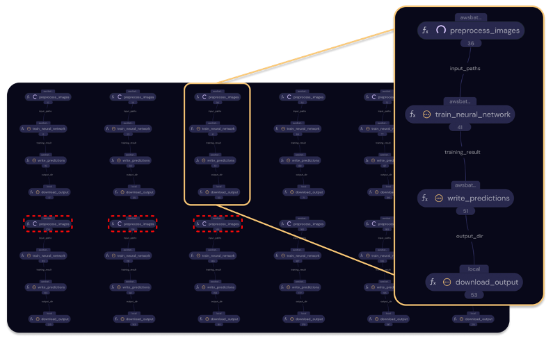
Figure 3 – Covalent UI showing concurrent execution of fully independent hyperparameter runs. This workflow is “naïve” (sub-optimal), because the several preprocessing nodes compute duplicate results. The dashed red lines in this figure outline one group of such nodes.

Covalent UI, naïve deployment strategy, group of four tasks for each independent run, nodes connected in simple linear order.

We deploy the workflow from a local script or Jupyter notebook by passing twelve combinations inside params_list when we dispatch the lattice. Covalent then uses awsbatch_exec to start the preprocessing task in every chain. When any of these tasks complete, the next adjacent task in Figure 3 is started in the same way. This continues until all tasks complete and the lattice function’s return value is assembled and returned.

We have thus created a distributed high-compute workflow that we can access directly from our local machine. Notably, this required no explicit containerization nor manual orchestration of our various tasks. Covalent also makes it easy to edit and refine our workflows. In fact, two important changes can make this experiment much more efficient.

Let’s improve this workflow and better highlight Covalent’s full potential.

Improved Deployment Strategy

By inspecting hp_sweep(), notice that we can reuse preprocessing results for hyperparameter runs over the same image size. We can modify the lattice function in any way we like, so long as only electrons are called from inside it. Below, to reduce the extra time (and cost) consumed by redundant preprocessing, we refactor hp_sweep() to preprocess once for each unique image size, and to later reference these results as required. Simply using a dictionary (inputs_dict) avoids unnecessary calls to preprocess_images() in this case:

@ct.lattice
def hp_sweep(data_dir: Path, params_list: List[Params], transform: Callable):
    inputs_dict = {}
    training_results = {}
    for i, ps in enumerate(params_list):

        if ps.image_size in inputs_dict:
           input_paths = inputs_dict[ps.image_size]
        else:
            input_paths = preprocess_images(data_dir, ps.image_size, transform)
            inputs_dict[ps.image_size] = input_paths  # save for next time

        training_result = train_neural_network(input_paths, ps, label=i + 1)
        output_dir = write_predictions(training_result)
        download_output(output_dir)

        training_result[ps] = training_result

    return training_results

A new transport graph visualizes this change. Note how the output of each preprocess_images() task is now shared among three dependent (i.e. connected) tasks.

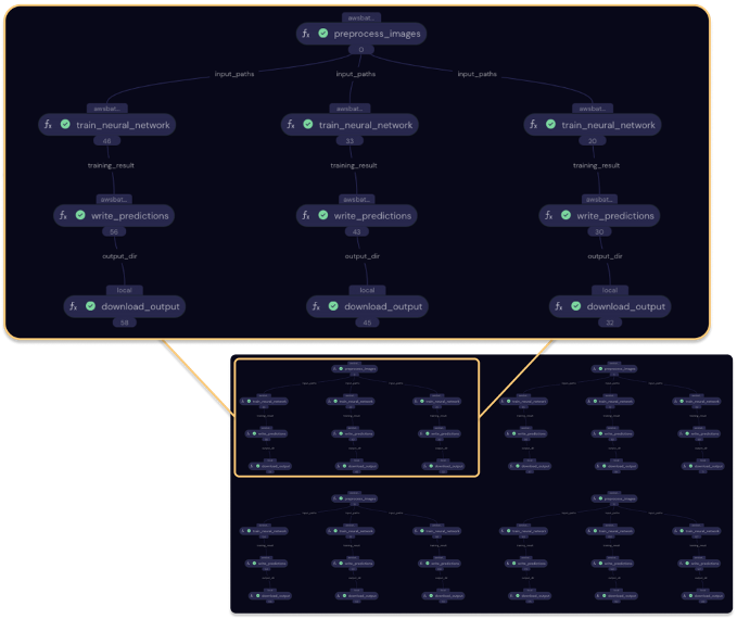
Figure 4 – Transport graph for the improved deployment, shown in completed state. The outlined sub-graph represents three hyperparameter runs that use the same preprocessing output.

Covalent UI, improved deployment strategy, preprocessing node result shared.

By refactoring the hp_sweep() function, we’ve also refactored our deployment strategy! This simple change has eliminated roughly two thirds of the preprocessing workload.

Distributing Across Multiple Instance Types

For a second improvement, we can defer all preprocessing tasks to a less powerful EC2 instance type, because preprocessing does not benefit from GPU acceleration. Suppose our compute environment can also launch Amazon EC2 R6a instances.  Recall that EC2 instance types are inferred from the AWS Batch executor’s parameters. Therefore, to make use of the R6a instances, we can define a second executor that requests zero GPUs by default:

import covalent as ct

# original executor for GPU instances
awsbatch_exec_gpu = ct.executor.AWSBatchExecutor(
    credentials="~/.aws/credentials",
    s3_bucket_name="my-s3-bucket",
    batch_queue="my-batch-queue",
    batch_job_log_group_name="my-log-group",
    time_limit=7200,
    vcpu=2,
    memory=4,
    num_gpus=1,
)

# create second executor to target R6a instances
awsbatch_exec_cpu = ct.executor.AWSBatchExecutor(
    credentials="~/.aws/credentials",
    s3_bucket_name="my-s3-bucket",
    batch_queue="my-batch-queue",
    batch_job_log_group_name="my-log-group",
    time_limit=3600,
    vcpu=2,
    memory=4,
)

# use `@ct.electron` to make electrons from individual tasks

@ct.electron(executor=awsbatch_exec_cpu)  # <-- update executor
def preprocess_images(data_dir, image_size, transform=None):
    """function that performs image preprocessing"""
    ...

@ct.electron(executor=awsbatch_exec_gpu)
def train_neural_network(input_paths, params, label):
    """function that runs the training/validation loop"""
    ...

@ct.electron(executor=awsbatch_exec_gpu)
def write_predictions(training_result):
    """function that tests the model against unseen data"""
    ...

@ct.electron(executor="local")  # execute in local process pool
def download_output(output_dir):
    """function that downloads prediction outputs from S3 bucket"""
    ...

Now, AWS Batch will launch an R6a instance (r6a.large) for every call to preprocess_images() from inside the lattice. Meanwhile, train_neural_network() and write_predictions() will run on P3 instances (p3.2xlarge) as before.

Results

Model Characterization

Using Covalent, we tested the improved workflow on the same twelve hyperparameter combinations (four different image sizes and three different learning rates). The results after twenty epochs are visualized below. In the 3D chart, we report the Sørensen-Dice coefficient between the model’s prediction and the correct segmentation area. This metric approaches 100% if and only if the predicted and true masks have the exact same shape and orientation. Four representative output images are also shown on the right-hand side of the figure below. While admittedly small, the experiment suggests that (1) the optimal learning rate is around 0.0001 and (2) that performance degrades significantly if the input images are reduced to a size below about 192 by 192 pixels.

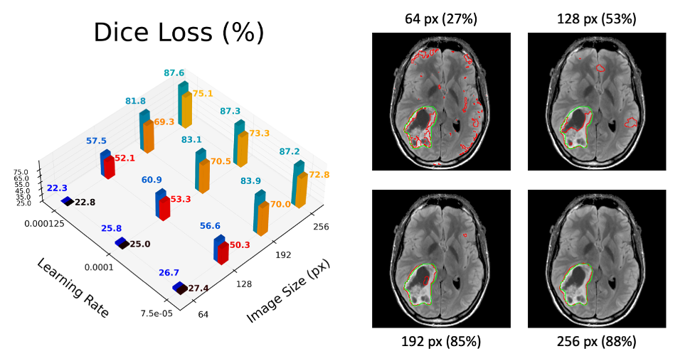
Figure 5 – Mean (black/red/yellow) and median (blue/teal) dice loss with typical results at each image size.

If the experimenter desires better predictions, they can immediately redeploy the workflow at any scale by dispatching the lattice with a new list of parameters. Further along, a new strategy can be implemented by editing hp_sweep(); for example, to incorporate any post-processing or to accept value ranges instead of an explicit parameter list. With Covalent, it’s always easy to undo these changes and we can always revisit older workflows in the Covalent UI.

Time and Cost Analysis

As a point of comparison, we repeated this experiment using a more traditional method, one which many practitioners employ when fast iteration is a priority. Since coordinating parallel execution over multiple instances is typically not suitable in this situation, the method in question involves running all twelve hyperparameter combinations serially, on a single p3.2xlarge instance—i.e. executing a Python script manually on a GPU instance. Although this results in a longer wall time compared to a parallel method using multiple instances, it also represents a lower bound in terms of compute hours and total charges. This is because the serial method avoids time overhead for multiple data transfers and instance startups.

In other words, we give the non-Covalent case the maximum possible advantage in this comparison, using a fast-iteration approach that is common among practitioners.

The final Covalent workflow is compared to this method in the figure below. The nominal cost of the Covalent deployment was less than $9 USD, versus nearly $25 USD without Covalent. These benefits come from the two improvements that we implemented above: namely, (1) avoiding redundant computations and (2) deferring to a lighter instance type for the remaining preprocessing tasks. Of course, both can in principle be achieved manually as well. However, Covalent significantly streamlines the creation of such workflows, as we hope to have demonstrated in this post so far.

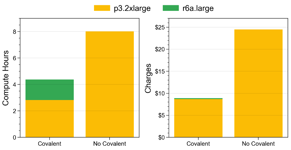
Figure 6 – Compute-hours and corresponding charges for the machine learning workflow; using Covalent versus manual execution. Both methods are suitable for quick, iterative experiments. However, Covalent makes it easy to create efficient deployments, leading to fewer computer hours and lower charges overall.

Covalent benefits figure, time saved, cost saved, comparison with standard serial method or an equivalent parallel method.

Conclusion

Using the Covalent SDK to orchestrate our cloud resources made the sample workflow twice as fast and 64% cheaper compared to the traditional method. These improvements can be attributed to Covalent’s design, which connects and scales the deployment strategy with the experimental logic, allowing users to easily build efficient solutions. Here, we achieved a 2x reduction in compute hours just by refactoring a simple loop. This lowered the overall cost, on top of significant savings gained by offloading preprocessing to a lighter instance type.

After the experiment, the final workflow remains fully reproducible, with all task results and metadata automatically cached in a scalable database. Future experiments can be run at any scale via different arguments for the lattice function, allowing practitioners to iterate without compromising efficiency. Because users aren’t saddled with manually interconnecting heterogenous resources, only a constant amount of effort is needed to further develop the deployment.

We hope this post has demonstrated Covalent’s potential when paired with powerful resources like AWS Batch. As a reminder, Covalent is free and open source. We encourage you to visit the Covalent Documentation for more information and many practical tutorials. Code for the sample implementation in this post can be found here.