AWS for Industries
Scalable Medical Computer Vision Model Training with Amazon SageMaker Part 2
Introduction
Training medical computer vision (CV) models requires a scalable compute and storage infrastructure. Training a medical CV model is unique compared to training a CV model in other domains, as we described in the first part of this blog series. In this second post, we show you how we scale a medical semantic segmentation training workload on terabytes of the BraTS brain tumor dataset from 90 hours to four hours. In our solution, we use Amazon SageMaker Processing for distributed data processing, Amazon FSx for Lustre for a high-performance file system, and the SageMaker distributed training library for faster model training. The data I/O, transformation, and network architecture are built using PyTorch and the Medical Open Network for AI (MONAI) library.
Solution Overview
Our solution to train a neural network with medical imaging at terabytes scale consists of the following Amazon Web Services (AWS):
- Amazon SageMaker (SageMaker) is a fully managed machine learning service. With SageMaker, data scientists and developers can quickly build and train machine learning models, and then directly deploy them into a production-ready hosted environment.
- Amazon SageMaker distributed training library, with only a few lines of additional code, can be used to achieve data parallelism or model parallelism to the training script. SageMaker optimizes the distributed training jobs through algorithms that are designed to fully utilize AWS compute and network infrastructure in order to achieve near-linear scaling efficiency, which allows you to complete training faster than manual implementations.
- Amazon SageMaker Processing provides a simplified, managed experience on SageMaker to run your data processing workloads, such as feature engineering, data validation, model evaluation, and model interpretation. Data preprocessing/transformation, as part of the data loading in training epochs, is a CPU heavy operation. If data preprocessing is run as part of the training epoch, it affects how quickly the CPU can transfer the data to the GPU to keep the GPU highly used. This then affects the overall runtime. It is therefore key to perform the data preprocessing beforehand.
- Amazon FSx for Lustre is a cost-effective way to launch and run the popular, high-performance Lustre file system. You use Lustre for workloads where speed matters, such as machine learning.
- MONAI is an open source project bringing medical imaging ML community together to create best practices of CV for medical imaging. It is built on top of a PyTorch framework and follows a native PyTorch programming paradigm, which is widely adopted. We use the data transformations and UNet model architecture from MONAI library.
At a high level, our proposed solution consists of three steps:
- A SageMaker Processing job to decompress, decode, scale, and augment I/O pairs and persist them on an Amazon Simple Storage Service (Amazon S3) before a model training job.

Figure 1. Sharded Image Transformation and Augmentation with Amazon SageMaker Processing
- Upon completion, the SageMaker distributed data processing job writes transformed data to a user specified Amazon S3 destination. To expedite data transfer from the Amazon S3 to the training hosts we create a high performant file system using Amazon FSx for Lustre.

Figure 2. High-performance file system for distributed data transfer using Amazon FSx for Lustre
- Lastly, launch a distributed data-parallel training job using the SageMaker SDK and SageMaker distributed training library. We will cover this in-depth later in this blog.
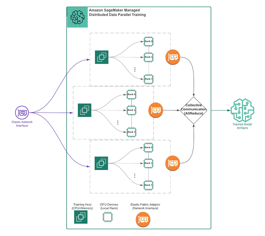
Figure 3. Distributed Data Parallel Training by Amazon SageMaker
Results
We ran the following experiments using the configurations listed in the table. Each training consists of 10 epochs. We measured the efficiency of a training job using epoch time in seconds. An epoch is a pass of the entire training dataset through the neural network during training. The table below summarizes the result.

Figure 4. Model training results showing training time improvement over various configurations
This is a 95% runtime improvement from about 90 hours to under four and a half hours. Note that the multi-GPU experiments (the second and third rows) include data preprocessing. Data preprocessing is done once. The output, which takes about 27 minutes, and the processed data can be reused in subsequent training experiments. Note that we did not aim to optimize for segmentation model accuracy.
Here is a step-by-step explanation on how to set up the solution to train a CV model at scale.
Prerequisite
Identity and Access Management (IAM) policy
To follow this example, you need AmazonSageMakerFullAccess permission in your IAM user as a baseline. To create an Amazon FSx for Lustre filesystem following the example below, you also need AmazonFSxFullAccess permission and additional permissions to use data repositories in Amazon S3 in your SageMaker execution role inside Amazon SageMaker Studio.
Amazon SageMaker Studio
Amazon SageMaker Studio (SageMaker Studio) is a web-based, integrated development environment (IDE) for machine learning that lets you build, train, debug, deploy, and monitor your machine learning models. To get started with SageMaker Studio, follow the Quick start procedure to onboard to SageMaker Studio in the account. Once the domain and a user profile are set up, open the SageMaker Studio. If this is your first time accessing the Studio, the JupyterServer setup will take a minute or two. Once in SageMaker Studio, open a system terminal from the launcher and run the following command to clone the code repository used in this blog.
$ git clone https://github.com/aws-samples/scalable-medical-computer-vision-with-amazon-sagemakerDataset
We use the dataset from the AWS Open Data Registry. Open the notebook 00-data_prep.ipynb and run the cells to get a copy of data both locally and to your SageMaker default Amazon S3 bucket in: s3://sagemaker-<region>-<account-id>/sagemaker-medical-imaging-blog/dataset/Task01_BrainTumour/ This process takes an hour.
Solution walkthrough
Image transformation with MONAI
MONAI is a medical imaging domain-specific library that offers a wide range of features and functionalities for medical imaging-specific data formats. Developers no longer need to write custom data loaders to process and train medical imaging data. You also do not lose any data integrity with unnecessary data conversion to other formats such as JPG or PNG. In addition, MONAI provides medical imaging-specific image processing as transformation and deep learning network architectures, which are proven in the medical imaging community. With this capability, developers don’t need to implement from scratch.
We construct transformation steps for the NIfTI image pair with the following transformation, which can be found in src/sharded_image_preprocessing.py:
# define transforms for image and segmentation
transforms = Compose(
    [
        # load 4 Nifti images and stack them together
        LoadImaged(keys=["image", "label"]),
        AsChannelFirstd(keys="image"),
        ConvertToMultiChannelBasedOnBratsClassesd(keys="label"),
        Spacingd(
            keys=["image", "label"],
            pixdim=(1.5, 1.5, 2.0),
            mode=("bilinear", "nearest"),
        ),
        Orientationd(keys=["image", "label"], axcodes="RAS"),
        RandSpatialCropd(
            keys=["image", "label"], roi_size=[128, 128, 64], random_size=False
        ),
        RandFlipd(keys=["image", "label"], prob=0.5, spatial_axis=0),
        NormalizeIntensityd(keys="image", nonzero=True, channel_wise=True),
        RandScaleIntensityd(keys="image", factors=0.1, prob=0.5),
        RandShiftIntensityd(keys="image", offsets=0.1, prob=0.5),
        ToTensord(keys=["image", "label"]),
    ]
)
Notably, MONAI’s transforms API supports dictionary-based data input and indexing. In medical imaging ML, it is typical to have image data and the label data saved in separate files. MONAI’s dictionary-based transforms (class name ending with -d, such as LoadImaged and RandFlipd) are suitable for this scenario. We can easily compose a chain of transformation for either the image or the label data with a key. In this transformation for training data we do the following (in the same order as in transforms):
- Load the NIfTI image pair as numpy arrays with the NIfTI headers associated.
- Make the image data channel first.
- Reconstruct the labels to create the aggregated labels: tumor core (TC), enhancing tumor (ET), and whole tumor (WT). This is a custom function.
- Resample the image and label data.
- Reorient both image and label data to RAS, which is the neurological convention.
- Randomly crop the image and label to reduce the size of the image and augment the data with randomness.
- Randomly flip the image and label on the first axis.
- Normalize the intensity of the image.
- Randomly scale the intensity of the image.
- Randomly shift the intensity of the image.
- Finally, convert the numpy arrays into tensors (still with the dictionary structure).
To run the preceding transformations as fast as possible, we use the multiprocessing library from Python to take advantage of all available CPU on each processing worker. This can be found in src/sharded_image_preprocessing.py:
def apply_transformations(file):
    output = transforms(file)
    output_name = file["image"].split('/')[-2] + '.pt'
    torch.save(output, os.path.join(output_dir, output_name))

pool = Pool(processes = cpu_count() - 2)
result = pool.map(apply_transformations, data_list)
Running an image preprocessing job on SageMaker Processing
In order to address data preprocessing bottlenecks, we use SageMaker Processing to perform both static and randomized transformations and persist the output on Amazon S3. The basic idea here is to reuse computation. That is, perform static or random transformations once, save on Amazon S3, and then use many times in one or multiple training jobs. Note that randomized preprocessing is usually part of the training loop itself. However, for the purpose of demonstrating the distributed data preprocessing capability of SageMaker Processing, we have factored out both static and randomized transformations from the training loop.
Note that with SageMaker Processing you can easily scale data preprocessing workloads either vertically (bigger compute instance) or horizontally (more compute instances). With horizontal scaling, SageMaker gives you the option to replicate the dataset fully on each worker node. Alternatively, you can shard the dataset into fragments to be divided evenly across a predefined number of worker nodes. Here we use SageMaker Processing to scale horizontally to 20 ml.c4.8.xlarge instances and by setting s3_data_distribution_type='ShardedByS3Key'. SageMaker automatically assigns ~2,444 (48,884/20) pairs to each processing worker. Furthermore, since each ml.c4.8.xlarge instance has 64 vCPUs, we use a process-based parallelism to map the transformation task across all CPUs on each worker node. This lets us process the 450 GB of compressed images in 27 minutes. You can find the following snippet in Step 1: SageMaker managed distributed image preprocessing in 01-model_training.ipynb.
from sagemaker.processing import ScriptProcessor
from sagemaker import get_execution_role

# Setup Processor
script_processor = ScriptProcessor(
    role=get_execution_role(),
    image_uri="763104351884.dkr.ecr.us-east-1.amazonaws.com/pytorch-training:1.8.1-cpu-py36-ubuntu18.04",
    instance_count=20,
    instance_type='ml.c4.8xlarge',
    volume_size_in_gb=1024
)

# Execute
from sagemaker.processing import ProcessingInput, ProcessingOutput
inputs = [ProcessingInput(source="s3://{}/{}/".format(bucket, input_prefix),
                          s3_data_distribution_type='ShardedByS3Key'
                         )
         ]

outputs = [ProcessingOutput(output_name='train',
                            destination="s3://{}/{}/".format(bucket, output_prefix),
                           )
          ]

date_time= strftime("%Y-%m-%d-%H-%M-%S", gmtime())
script_processor.run(job_name="monai-transforms-sharded-{}".format(date_time),
                     code='src/sharded_augmentation.py',
                     inputs=inputs,
                     outputs=outputs,
                     wait=False
                    )
Set up an Amazon FSx for Lustre file system with the processed dataset
In order to deal with the networking bottleneck during the data I/O step in the training loop, we use Amazon FSx for Lustre. It provides enough throughput for multiple GPU hosts to read the processed data from Amazon S3 in parallel. To set up Amazon FSx for Lustre, you can run a single command using AWS SDK for Python (boto3). Storage capacity starts at 1.2 TiB or 2.4 TiB and can be scaled up in increments of 2.4 TiB with proportional throughput. Note that the file system must be in the same Amazon Virtual Private Cloud (Amazon VPC) subnet that is used for model training. You can find the following snippet in Step 2: Amazon FSx for Lustre in 01-model_training.ipynb.
fsx_client = boto3.client("fsx")

fsx_response = fsx_client.create_file_system(
    FileSystemType='LUSTRE',
    StorageCapacity=2400,
    StorageType='SSD',
    SubnetIds=[vpc_subnet_ids[0]],
    SecurityGroupIds=security_group_ids,
    LustreConfiguration={
        'ImportPath': processing_output_path,
        'DeploymentType': 'PERSISTENT_1',
        'PerUnitStorageThroughput': 200
    }
)
Building a training script with MONAI
Next, we create a training script that can later be used in SageMaker’s fully managed training infrastructure. We first use a custom PyTorch dataset to load augmented images and labels. You can find the following snippet in src/multi_gpu_training.py.
class ProcessedDataset(Dataset):
    def __init__(self, data_list):
        self.data_list = data_list

    def __len__(self):
        return len(self.data_list)

    def __getitem__(self, index):
        file_path = self.data_list[index]
        file = torch.load(file_path)
        image = file['image']
        label = file['label']
        return (image, label)

# split the data_list into train and val
data_list = sorted(glob(os.path.join(args.train, '*.pt')))
train_files, val_files = partition_dataset(
    data_list,
    ratios=[0.99, 0.01],
    shuffle=True,
    seed=args.seed
)

# create training/validation datasets / dataloaders
train_ds = ProcessedDataset(data_list=train_files)
val_ds = ProcessedDataset(data_list=val_files)

train_loader = DataLoader(
    train_ds,
    batch_size=args.batch_size,
    shuffle=False,
    num_workers=args.num_workers
)
val_loader = DataLoader(
    val_ds,
    batch_size=args.batch_size,
    shuffle=False,
    num_workers=args.num_workers
)
For the semantic segmentation model, we use the UNet implementation from MONAI. Note that the input data is a three-dimensional image with four modalities (channels).
model = monai.networks.nets.UNet(
    dimensions=3,
    in_channels=4, # BraTS data has 4 channels (modalities)
    out_channels=3,
    channels=(16, 32, 64, 128, 256),
    strides=(2, 2, 2, 2),
    num_res_units=2,
)
With the dataset, data loader, and model defined, we create a trainer as a utility function to perform the model training. Then we can train with SageMaker’s fully managed training infrastructure.
Training with SageMaker Managed Training
In the training notebook 01-model_training.ipynb, we use the PyTorch estimator from SageMaker Python SDK and bring in the training code using the script mode. The following snippet shows how to start a single node training job in SageMaker for the script src/single_gpu_training.py.
instance_type = 'ml.p3.2xlarge'
instance_count = 1
training_input = "s3://{}/datasets/Task01_BrainTumour/".format(bucket)

estimator = PyTorch(
    role=role,
    sagemaker_session=session,
    source_dir='src',
    entry_point='single_gpu_training.py',
    hyperparameters=hyperparameters,
    py_version='py36',
    framework_version='1.6.0',
    ...
    instance_count=instance_count,
    instance_type=instance_type
)

estimator.fit(
    job_name='unet-brats-training-{}'.format(job_tag),
    inputs={'train':training_input}
)
Note that we provide training code as the entry_point with source_dir to the PyTorch estimator. The library dependency (MONAI and others) for the training code should be listed with a requirements.txt file located in the source_dir.
SageMaker estimators help you choose the compute resource needed for the job. You can choose which compute resource you’d like to use as part of the estimator construct with instance_count and instance_type. In the preceding code snippet, one ml.p3.2xlarge instance was shown as an example, which has one NVIDIA Tesla V100 GPU with 16-GiB GPU memory. With this setup we can achieve the first training runtime in the preceding results section, that is, a 31,000 epoch time on one ml.p3.2xlarge instance. This is unfortunately not an efficient solution, as it would take four days to complete a 10-epoch training.
Let’s examine distributed training next. The SageMaker distributed training library enables your training code to work with multiple GPU devices (either in one or multiple instances) efficiently.
SageMaker distributed data parallel training
In this section we show how to distribute the previous training job across multiple GPU devices. Each device is assigned a single process. Each process performs the same task (forward and backward passes) on different shards of data. That is, we show how to use SageMaker’s distributed data parallel (SMDDP) library. Note that SageMaker also supports distributed model parallel training.
Adopting SMDDP requires only a few changes to our training script. To start, we initialize a distributed processing group and set each GPU to a single process. We also import the SageMaker DistributedDataParallel class, which is an implementation of distributed data parallelism (DDP) for PyTorch. You can find the following snippets in src/multi_gpu_training.py.
import torch
import smdistributed.dataparallel.torch.distributed as dist
from smdistributed.dataparallel.torch.parallel.distributed import DistributedDataParallel

# initialize the distributed training processing group
dist.init_process_group()

# pin each GPU to a single process
torch.cuda.set_device(dist.get_local_rank())
Next, we replicate our data loader across our group of processes using PyTorch’s DistributedSampler. The number of replicas is set via num_replicas=arg.world_size and each replica is assigned a rank within the group.
from torch.utils.data.distributed import DistributedSampler
train_loader = DataLoader(
    train_ds,
    batch_size=args.batch_size,
    shuffle=False,
    num_workers=args.num_workers,
    sampler=DistributedSampler(train_ds,
                              num_replicas=args.world_size,
                              rank=args.host_rank)
 )
The model definition does not need to change. We do, however, need to wrap the model with the SageMaker DistributedDataParallel class. This grants each process its own copy of the model so it can perform the forward and backward passes on its subset of each batch of data.
# wrap the model with sm DistributedDataParallel module
model = DistributedDataParallel(model)
Lastly, we save checkpoints only on the leader node in the trainer. This is done with an if-statement in the training loop:
if dist.get_rank() == 0:
    torch.save(
        model.state_dict(),
        os.path.join(args.model_dir, "best_model.pth")
        )
These are the only changes we need to make to our entry point script. Now, back to the 01-model_training.ipynb notebook, in order to execute this updated entry point, we must activate the distribution option in the SageMaker’s PyTorch estimator:
estimator = PyTorch(
    ...
    entry_point='multi_gpu_training.py',
    instance_count=instance_count,
    instance_type=instance_type,
    distribution={'smdistributed': {'dataparallel': {'enabled': True}}}
)
By setting instance_count=1 and instance_type='ml.p3.16xlarge', we would get a runtime performance of around 2,400 seconds per epoch. If we scale out to instance_count=2 using the same instance type, we would get a runtime performance of around 1,300 seconds per epoch, as shown in the results section.
Clean Up
To avoid resources incurring charges, remove the data in the Amazon S3 bucket, the Amazon FSx for Lustre file system, and the kernel gateway apps from SageMaker Studio. Instances behind SageMaker Processing and SageMaker training jobs are automatically shut down at the end of the jobs.
Conclusion
In this blog post, we demonstrated a scalable model training solution for a multi-modality MRI brain tumor dataset that we augmented to terabyte size. We used MONAI library for its medical imaging data I/O, transformation, and network architecture to build out our model training script.
We showed you the architecture based on the following SageMaker capabilities: managed training, distributed data parallel, and processing with an Amazon FSx for Lustre file system to achieve a desirable high network throughput. We benchmarked the model training runtime performance on the scaled dataset with various compute infrastructure setups.
The benchmark results showed that by using the architecture, we were able to achieve a runtime reduction from 90 hours to four hours for the terabyte-scale dataset. The solution is transferrable to other imaging modalities such as lung computed tomography, lung X-Ray, skin dermatoscopy, and digital pathology once the data size exceeds the capacity of a single machine.
With this scalable solution, data scientists working in the healthcare and life science domain can train medical imaging models with larger datasets and richer information from multi-modality imaging techniques. ML teams can iterate faster over model tuning, resulting in a more accurate model. This, in turn, would help researchers, radiologists, clinicians, and healthcare providers understand disease patterns better and provide more personalized treatment.