Analog Hamiltonian simulation with PennyLane

We are excited to announce that customers can now run analog Hamiltonian simulation (AHS) on Rydberg atom quantum devices on Amazon Braket, via the Braket-Pennylane plugin. Rydberg atom devices, such as QuEra’s Aquila, are a type of neutral-atom quantum computer which features customizable qubit geometry and time-dependent parameter control, allowing you to control the system’s quantum evolution with high precision. In addition to being well-suited to solving optimization problems, AHS provides the ability to explore highly entangled systems, for instance, quantum phases of matter.

When designing the AHS program however, searching for the optimal parameters to implement such a simulation can be tedious. With this launch, users can leverage the quantum machine learning techniques from PennyLane to optimize the AHS programs for the Rydberg atom device.

In this post, we will describe how you can use the Braket-Pennylane plugin to study the ground state of the anti-ferromagnetic Ising spin-chain on a 1D lattice on the Aquila quantum processor, a neutral-atom quantum computer available on-demand via the AWS Cloud.

Analog Hamiltonian simulation with Rydberg atoms

AHS is an approach to studying the properties of a quantum system by tuning the parameters of another quantum system which closely resembles the first. In an AHS program, we first need to find a set of parameters which minimize the cost function we’re interested in. For this task, various optimization methods have been studied in the AHS literature, including stochastic optimizers, Bayesian optimizations, and more. In this blog post, we demonstrate how to optimize the parameters for Rydberg atom devices using differentiable programming techniques included in PennyLane.

As an example, we’ll consider a chain with nine spins, each of which can be in “up” or “down” states. We are interested in studying the so-called anti-ferromagnetic (AFM) order, a naturally occurring phenomena in magnetic materials, where neighboring spins point in opposite directions. To simulate the spin chain, we map each spin to an atom, with the ground and excited Rydberg states of each atom corresponding to “down” and “up” spins, respectively. With this encoding, the AFM order of interest corresponds to an alternating pattern of ground and Rydberg states for the chain of nine atoms.

Using PennyLane, we will first create an arrangement with nine atoms by explicitly specifying their coordinates:

# For realizing the AFM order, the atomic spacing is typically
# chosen between 6 and 7 micrometers. The interested readers are
# encouraged to try other values of atomic spacing!
a = 6.1 # μm
num_atoms = 9
coords = []
for k in range(num_atoms):
    coords.append([k * a, 0])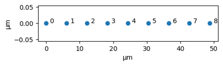

Figure 1: A plot of the positions of nine atoms in a spin chain in micrometers

At the beginning of the AHS program, all the atoms are initialized in the ground state; we then aim to tune the time-dependent parameters of the system, including the amplitude of the Rabi frequency and detuning, to drive the system to the AFM state.

You can see an example of this in our ordered phases AHS example notebook, where the time-series of the driving fields are specified as discrete sets of time-value pairs. Here, on the other hand, we will specify the time-series of the driving fields as continuous, differentiable functions.

Creating differentiable Hamiltonians with PennyLane

To create a differentiable driving field, we will first specify some constraints, such as the maximum allowed values for amplitude and detuning: two of the three time series that make up the AHS driving field.

import pennylane.numpy as np

amplitude_max = 1.58e7 # rad/second
detuning_max = 1.25e8 # rad/second
time_max = 4e-6 # second
C6 = 862619.79 # MHz μm^6

def angular_SI_to_MHz(angular_SI):
    """Converts a value in rad/s or (rad/s)/s into MHz or MHz/s"""
    return angular_SI / (2 * np.pi) * 1e-6

time_max = time_max * 1e6 
amplitude_max = angular_SI_to_MHz(amplitude_max)
detuning_max = angular_SI_to_MHz(detuning_max)

print(f"amplitude_max    = {round(amplitude_max, 2)} MHz")
print(f"detuning_max = {round(detuning_max, 2)} MHz")
print(f"time_max     = {time_max} μs")

Out:
amplitude_max    = 2.51 MHz
detuning_max = 19.89 MHz
time_max     = 4.0 μs

Here we have limited the maximum duration of the program, time_max, to be 4μs, and introduced the Rydberg interaction constant C₆. These constants are specific to QuEra’s Aquila at time of writing, and in general they can be queried from the Braket SDK as shown in our intro to Aquila AHS example notebook. With these constants, the differentiable driving fields for the Rydberg atom device can be defined via PennyLane’s JAX scientific computing library.

import jax.numpy as jnp
import jax

# Set to float64 precision and remove jax CPU/GPU warning
jax.config.update("jax_enable_x64", True)
jax.config.update("jax_platform_name", "cpu")
jax.config.update("jax_debug_nans", True)

def ryd_amplitude(p, t):
    """Parametrized function for amplitude"""
    return p[0] * (1-(1-jnp.sin(jnp.pi * t/time_max)**2)**(p[1]/2))

def ryd_detuning(p, t):
    """Parametrized function for detuning"""
    return p[0] * jnp.arctan(p[1] * (t-time_max/2)) / (jnp.pi/2)

Important: firstly, mathematical functions, such as trigonometric functions, should be explicitly defined as JAX functions for them to be differentiable; secondly, the callable functions, such as ryd_amplitude, should have signature (p, t), which is required when defining the ParametrizedHamiltonian object for the Rydberg atom device (see H_ryd below).

The function ryd_amplitude starts and ends at zero, as required for the amplitude of the Rabi frequency for QuEra’s Aquila. We start the detuning, as parametrized by ryd_detuning, at a negative value to ensure that the initial state (where all atoms are in the ground state) is the lowest energy state of the Hamiltonian. As we gradually increase the detuning to a positive value, the Rydberg system is adiabatically driven to the AFM order. As an example, we define a set of parameters for the driving fields:

vis_time = np.linspace(0, time_max, 100)

# These parameters are chosen arbitrarily for demonstration purpose.
# The readers are interested to try out other parameters!
amplitude_para = [amplitude_max, 10]
detuning_para = [detuning_max * 2/3, 1.45]

Which we can plot as follows:

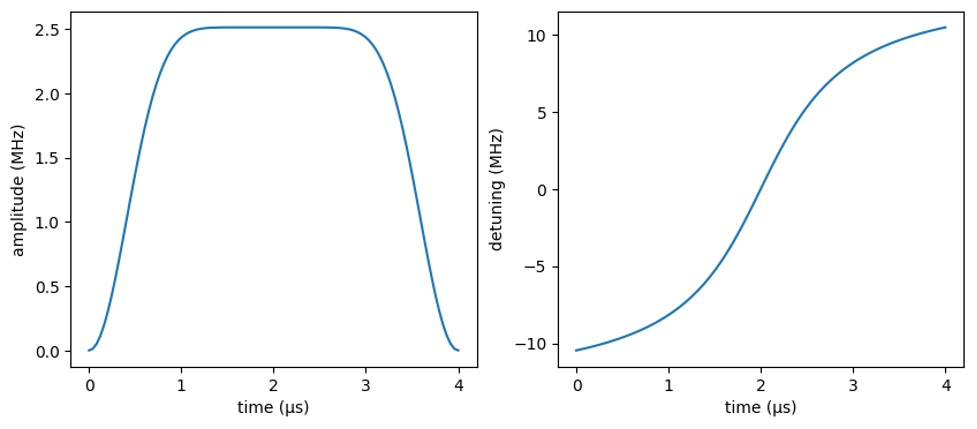
Figure 2: The adiabatic evolution of amplitude and detuning values over the course of driving

We now construct the parametrized function for the global driving field for the Rydberg atoms out of the amplitude and detuning functions:

import pennylane as qml

global_drive = qml.pulse.rydberg_drive(amplitude=ryd_amplitude,
                                       phase=0,
                                       detuning=ryd_detuning,
                                       wires=range(len(coords)))

In this example, for simplicity we have fixed the phase, another time-dependent parameter for Rydberg devices, to be zero. Finally, the full Rydberg Hamiltonian is the sum of the driving field and the Rydberg interaction. 

H_ryd = global_drive + qml.pulse.rydberg_interaction(coords, interaction_coeff=C6)

Simulating anti-ferromagnetic order with Rydberg atoms

So, we created a time-dependent, parameterized Rydberg Hamiltonian. Now let’s see if it can realize the AFM order. For that, we’ll define the following parametrized AHS program:

ts = [0, time_max]

def program(detuning_para, amplitude_para = amplitude_para, ts = ts):
    qml.evolve(H_ryd)([amplitude_para, detuning_para], ts)
    return qml.counts()

Here qml.evolve returns a ParametrizedEvolution object which has the same set of parameters as the parametrized Hamiltonian H_ryd. The program takes in the parameters for detuning and outputs the measurement outcome of the AHS program. Below, we will optimize the detuning parameters, while keeping those for the amplitude fixed. The AHS program can be run on the PennyLane simulator as follows:

shots = 1000

# Introduce the PennyLane local simulator
simulator_pl = qml.device("default.qubit.jax", wires=len(coords), shots=shots)

# Define the qnode that runs the AHS program
program_pl = qml.QNode(program, simulator_pl, interface="jax")

# Run the program with a specific set of parameters for the detuning
counts_pl = program_pl(detuning_para)

We’ll then plot the probability of Rydberg state for each site, averaged over all the shots:

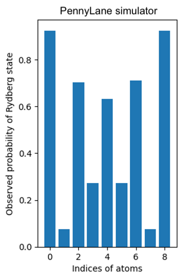
Figure 3: Observed probability of Rydberg atom occupancy by index for the PennyLane AHS simulator

In the following, we will focus on the PennyLane local simulator, which supports the JAX interface for differentiable programming.

For a chain of atoms, the average Rydberg probability of the ideal AFM order forms an alternating pattern of zeros and ones. In particular, atoms in the odd-index and even-index sites tend to be in the ground and Rydberg states, respectively. From the preceding plots, we see that the AHS program approximately produces the AFM state of interest. The discrepancy, which is more prominent at the center of the chain, can be attributed to the non-adiabaticity during the evolution. We can improve the AFM order further by tuning the detuning field, but doing this manually by searching through the parameter space is expensive. We will now show that the differentiable programming can be helpful in this scenario.

Cost function for anti-ferromagnetic order

To optimize the AHS program, we need to define a cost function, which characterizes the “quality” of the AFM order. The cost function is defined as follows:

We will use binary variables x_i to represent the states of the atoms:x_i=1 when the i-th atom is in the Rydberg state, otherwise x_i=0. When two neighboring atoms occupy ground and Rydberg states respectively, they form a domain wall, and the preceding cost function counts the number of domain walls in the atomic chain. For an ideal AFM order, each domain wall contributes -1/4 to the cost function, and for the nine-atom chain, this sums up to H_cost=-2.

The cost function can be specified as follows.

# Initialize the cost function
H_cost = 0
for i in range(len(coords)-2):
    # Add the contribution from each domain wall
    H_cost += qml.prod(qml.Projector([1], wires=[i]) - 1/2, qml.Projector([1], wires=[i+1]) -1/2)

Here we use the Projector in PennyLane to represent the Boolean variables. For example, qml.Projector([0], wires=[1]) represents x₁=0 and qml.Projector([1], wires=[2]) represents x₂=1. The product between the Boolean variables is realized with qml.prod.

Variational analog Hamiltonian simulation program with PennyLane

With the cost Hamiltonian defined, we can create a variational AHS program, which evolves the Rydberg system followed by measuring the cost function H_cost.

# Define the PennyLane local simulator
dev = qml.device("default.qubit.jax", wires=range(len(coords)))

# Define the qnode that evolves the Rydberg system, followed by calculating the cost function
@qml.qnode(dev, interface="jax")
def program_cost(detuning_para, amplitude_para = amplitude_para, ts = ts):
    qml.evolve(H_ryd)([amplitude_para, detuning_para], ts)
    return qml.expval(H_cost)

We note that program_cost is a parametrized AHS program that has only one positional argument, the parameters for the detuning, and outputs the cost function H_cost. With the JAX interface, we can optimize the detuning to minimize the cost function. We use detuning_para defined previously as the initial parameter for the optimization.

theta = detuning_para.copy() 
initial_cost = program_cost(theta)
print(f"The initial parameter for detuning = {theta}")
print(f"The initial cost = {initial_cost}")

Out:
The initial parameter for detuning = [13.262911924324612, 1.45]
The initial cost = -1.4220786805245211

We see that the initial cost function ≈-1.422, which is larger than the expected value for the ideal AFM order: -2. This is consistent with our finding that the corresponding state is not an ideal AFM order. To minimize the cost function H_cost, we first introduce a JAX function that calculates the expectation value and its gradient:

value_and_grad = jax.jit(jax.value_and_grad(program_cost))

# Compile the value_and_grad function
_, _ = value_and_grad(theta)

Next, we define the learning rate schedule, followed by using the adam implementation in optax for optimization.

import optax

n_epochs = 10

# The following block creates a constant schedule of the learning rate
# that increases from 0.1 to 0.5 after 10 epochs
schedule0 = optax.constant_schedule(1e-1)
schedule1 = optax.constant_schedule(5e-1)
schedule = optax.join_schedules([schedule0, schedule1], [10])
optimizer = optax.adam(learning_rate=schedule)
opt_state = optimizer.init(theta)

Now we are ready to run the optimization.

energy = np.zeros(n_epochs + 1)
energy[0] = program_cost(theta)
gradients = np.zeros(n_epochs)

## Optimization loop
print("epoch  expectation")
for n in range(n_epochs):
    val, grad_program = value_and_grad(theta)
    updates, opt_state = optimizer.update(grad_program, opt_state)
    theta = optax.apply_updates(theta, updates)

    energy[n + 1] = val
    gradients[n] = np.mean(np.abs(grad_program))

    print(n, "   ", val)
    
print(f"The final parameter for detuning = {[float(i) for i in theta]}")

Out:
epoch  expectation
0     -1.4220786805245298
1     -1.4440255545399932
2     -1.4682669156813462
3     -1.4949299366493178
4     -1.5241454186166363
5     -1.5561124234486559
6     -1.5902746804696113
7     -1.6261105967626694
8     -1.6618436930216522
9     -1.6951979675012514

The final parameter for detuning = [12.268508609204051, 0.435397311519117]

We see that the expectation H_cost is indeed gradually decreasing, as expected. In order to reach the expected value -2, we encourage interested readers to try larger number of epochs or different optimization schedules. By construction, a larger absolute value of H_cost corresponds to a sharper alternating pattern for the Rydberg probability. To confirm that, we calculate the Rydberg probability with the optimized detuning, followed by comparing the Rydberg probability before and after the optimization.

Plotting which gives us:

# Run the program with the optimized parameters for the detuning
counts_pl_optimized = program_pl(theta)
# Calculate the Rydberg density averaged over all the shots
prob_pl_optimized = get_prob(counts_pl_optimized)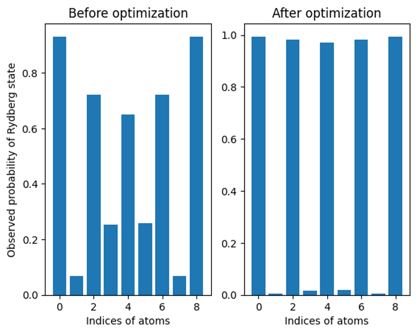

Figure 4: Observed probability of Rydberg atom occupancy by index for the PennyLane pre- and post-optimization (simulated data)

Indeed, the AFM order after optimization exhibits a sharper alternating pattern compared to that before the optimization. We can also compare the detuning before and after the optimization, as follows:

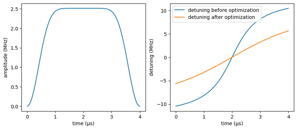
Figure 5: The adiabatic evolution of amplitude and detuning values over the course of driving, with optimized detuning shown right

The optimized detuning exhibits a smaller slope, particularly in the middle of the evolution, compared to that before the optimization. A less steep slope is desirable here, since we want to maintain adiabaticity during our full quantum evolution, and indeed the optimized version produces the almost ideal AFM order.

Running on a real neutral-atom quantum computer

To illustrate the usefulness of optimizing the AHS program, we’ll run the two AHS programs, before and after the optimization, on QuEra’s Aquila device and compare the results, the code for which is as follows:

aquila = qml.device(
    "braket.aws.ahs",
    device_arn="arn:aws:braket:us-east-1::device/qpu/quera/Aquila",
    wires=len(coords),
)

program_cost_aquila = qml.QNode(program, aquila)

counts_aquila_before = program_cost_aquila(detuning_para)
counts_aquila_after = program_cost_aquila(theta)

In between these steps, we need to do some simple pre-processing, the details for which you can review in this blog’s companion notebook. Next, we’ll get the probabilities:

prob_aquila_before = get_prob(counts_aquila_before)
prob_aquila_after = get_prob(counts_aquila_after)

Which we can plot as follows:

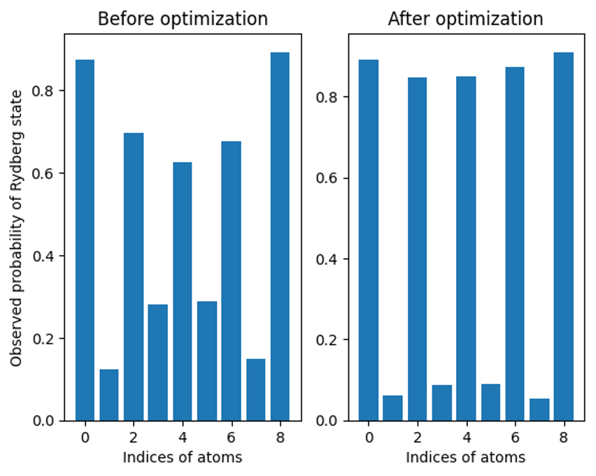
Figure 6: Observed probability of Rydberg atom occupancy by index for the PennyLane pre- and post-optimization (device data)

We find that the optimized AHS program when run on the real device indeed yields an AFM order that is much closer to an ideal one, compared to the non-optimized AHS program. This suggests that for AHS programs with small number of atoms, optimizing on the local simulator with PennyLane before submitting to the actual hardware is an effective way to make better use of the near-term quantum hardware in this case.

Note: running on the Aquila system will incur a cost, and readers are encouraged to review our pricing page for more details. With Amazon Braket, you only pay for what you use, with no upfront costs or commitments.

Conclusion

In this blog, we announced support for analog Hamiltonian simulation via the Braket-Pennylane plugin. Customers can now use differentiable techniques from machine learning to optimize the parameters of their AHS programs for neutral-atom systems, accelerating research in quantum computing.

To further enable experimentation, we recently expanded the availability of QuEra’s Aquila on Braket by 10x. With this expansion, we’re providing customers all over the globe with 100hrs of on-demand access to a neutral-atom QPU.

We also encourage interested readers to try to come up with different parametrizations for the driving field, which may be useful to realize other phases of matter with Rydberg atoms. To get started, try out the demo notebook. To learn more about using QuEra’s Aquila system to study problems in optimization, check out our blog.

Researchers can apply for credits via the AWS Cloud Credit for Research program.