AWS Quantum Technologies Blog
Introducing the Qiskit provider for Amazon Braket
We are excited to share a solution to one of our most frequent customer requests: a Qiskit provider for Amazon Braket. Users can now take their existing algorithms written in Qiskit, a widely used open-source quantum programming SDK and, with a few lines of code, run them directly on Amazon Braket. The qiskit-braket-provider currently supports access to superconducting quantum processing units (QPUs) from Rigetti and Oxford Quantum Circuits, an ion trap QPU from IonQ, as well as Braket’s on-demand simulators: SV1, TN1, and DM1.
The qiskit-braket-provider was developed primarily by open-source contributor David Morcuende as part of the Qiskit Advocate Mentorship Program, in collaboration with the Amazon Braket team. Encouraging this type of project is exactly why the Braket Python SDK and Braket Examples GitHub repos are open-source: we want to empower everyone in the quantum computing community to contribute to and influence the future of the field. Contributors can define which quantum algorithm or software feature examples they want to see, which tools or plugins would make their quantum application development easier – even invent new quantum algorithms. If you have an idea for an open-source project around Amazon Braket, we invite you to submit an issue in our Braket examples repo or Braket Python SDK repo, and you may end up creating a tool like the qiskit-braket-provider.
How to run your Qiskit code on Braket quantum devices
In this tutorial, you will learn how to run a Qiskit circuit to create an entangled qubit state on multiple different QPUs available on Amazon Braket from your local machine, either in a Jupyter notebook or in your favorite IDE. You can also use a Braket managed notebook by following this guide and installing the qiskit-braket-provider via pip.
Setup and installation
If you don’t have an AWS account, or you’re an AWS user but haven’t used Amazon Braket before, you’ll need to set up your local development environment to be able to access Braket resources like QPUs, which you can do by following steps 1-5 of this tutorial. After you’ve completed this setup, you should have 1) an AWS account, 2) an AWS access key ID and secret access key, 3) the Braket service and third-party devices (QPUs) enabled, 4) the AWS Command Line Interface (CLI) installed and configured to allow programmatic access to AWS resources, and 5) the Amazon Braket SDK pip installed in your local environment.
Next, you’ll pip install the qiskit-braket-provider in your local environment from your terminal:
To make sure the provider has been installed properly, you can start up Python and try importing the library:
If the provider was installed correctly, this should return the prompt back with an empty output. Now, you are ready to create your quantum program.
Creating entangled qubit states with Qiskit
A common “Hello, World!” program for quantum computers is creating a Bell state: a two-qubit entangled state. When we entangle more qubits together in the same way, we can create what’s called a GHZ state. Below we show how you can use the qiskit-braket-provider to run circuits against multiple backends on Amazon Braket. In Qiskit, the code for a 3 qubit GHZ state is as follows:
from qiskit import QuantumCircuit

circuit = QuantumCircuit(3)

# Apply H-gate to the first qubit:
circuit.h(0)


# Apply a CNOT to each qubit:
for qubit in range(1, 3):

    circuit.cx(0, qubit)
We can visualize the circuit by calling
circuit.draw('mpl')
In this circuit, we first put qubit 0 into superposition by acting on it with the Hadamard gate, then we perform a controlled X gate from qubit 0 onto the other two qubits, which entangles all the qubits together. If we run a simulation of this circuit, we will always get measurement outcomes that are perfectly correlated: roughly half the time all qubits will be 0, and the other half all qubits will be 1. Because quantum mechanics is inherently probabilistic, the more times we re-run the circuit (the number of “shots”), the closer we will get to precisely half 000 and half 111 states. We can run this circuit on the Braket local simulator via the qiskit-braket-provider for 1000 shots:
from qiskit_braket_provider import BraketLocalBackend

local_simulator = BraketLocalBackend()

task = local_simulator.run(circuit, shots=1000)
To see the measurement outcomes, we will use a convenient plotting function from Qiskit to plot the probability of measuring each state:
from qiskit.visualization import plot_histogram

plot_histogram(task.result().get_counts())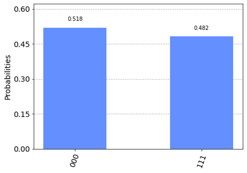
As expected, we only see states where the qubits are all 0 or all 1, in a roughly 50-50 split.
Running your circuit on real quantum computers
If we want to run a GHZ circuit on a real quantum computer (or several), we only need to specify the backend:
from qiskit_braket_provider import AWSBraketProvider

provider = AWSBraketProvider()

# devices
ionq_device = provider.get_backend("IonQ Device")

rigetti_device = provider.get_backend("Aspen-M-1")

oqc_device = provider.get_backend("Lucy")
Here we have access to an ion trap QPU and two superconducting QPUs. Because the quantum devices are not available 24/7, Braket queues the task for you and runs it when the QPU is available. You can access your results using the task’s Amazon Resource Name (ARN). NOTE: running on real quantum computers will incur costs on your AWS account. If you are a student or researcher, considering applying for AWS Cloud Credits for Research.
ionq_task = ionq_device.run(circuit, shots=100)

ionq_arn = ionq_task.job_id()![]()
Note: Amazon Braket uses the term Job to refer to a Hybrid Job, which is a feature of the Braket service that provides optimized quantum-classical workload orchestration for variational quantum algorithms. Qiskit uses the term “job” to refer to what is called a task in Amazon Braket. The single circuit that we are running multiple shots of in this tutorial is therefore considered a task in the language of Braket and a “job” in the language of Qiskit.
We can retrieve our task by its ARN and check its status:
ionq_retrieved = ionq_device.retrieve_job(job_id=ionq_arn)

ionq_retrieved.status()![]()
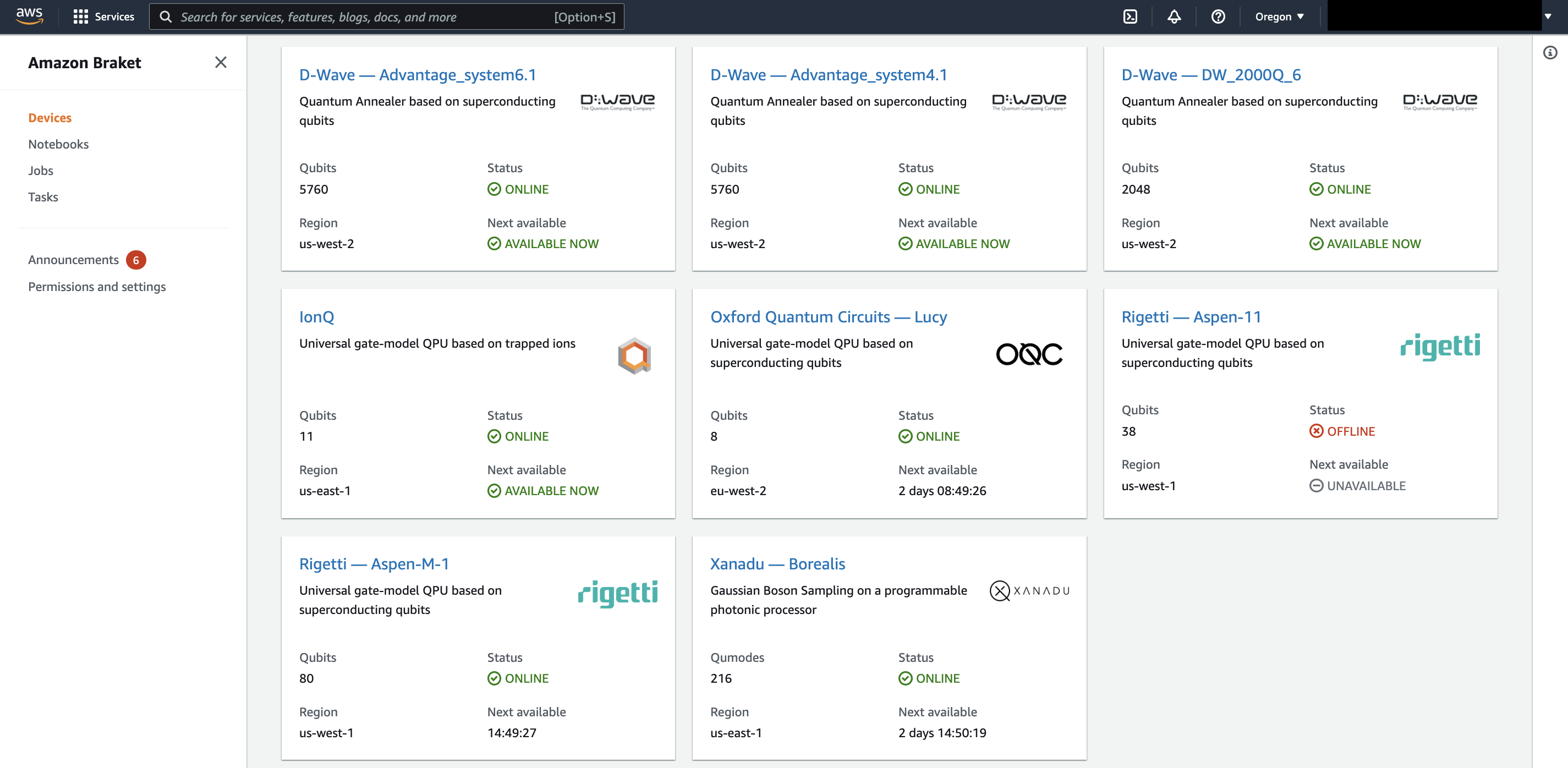
Check the Devices page on the Braket console to see when the QPU will next be available for an estimate of when your task will be processed.
When our task is completed, the retrieved_task.status() will be “Done:”
![]()
To receive a notification via Amazon EventBridge when the task is completed, you can follow this tutorial.
Now we can plot the measurements results just like we did with the simulated task:
plot_histogram(retrieved_job.result().get_counts())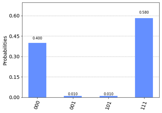
In a real quantum computer, there is noise, so we see states other than the ideal 000 and 111 GHZ state. Additionally, either due to the noise or because we used a lower number of shots (100), the measurement statistics are further from the 50-50 split that quantum mechanics predicts. Still, we have successfully created entanglement in an ion trap in Maryland!
Next we will run the same circuit on the Rigetti Aspen-M-1 superconducting quantum computer. This device has 80 qubits, but we’ll only be using 3 for our demo.
rigetti_task = rigetti_device.run(circuit, shots=100)

# retrieve task by ID
rigetti_retrieved = rigetti_device.retrieve_job(job_id=rigetti_task.job_id())
Again, we may need to wait for our measurement results and come back later. The status for a given task is available via the same API, regardless of which QPU we run on: rigetti_retrieved.status()
When the task is completed, we can plot the results exactly the same way:
# plot results
plot_histogram(rigetti_retrieved.result().get_counts()) 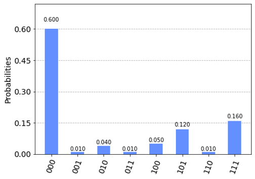
In this plot, we see a different distribution of output states because of the differences in hardware and their inherent noise characteristics.
Finally, we’ll create our GHZ state on the Oxford Quantum Circuits (OQC) superconducting device: “Lucy.” Switching between Rigetti and OQC only requires you to change a single line of code:
oqc_task = oqc_device.run(circuit, shots=100)

# retrieve task by ID
oqc_retrieved = oqc_device.retrieve_job(job_id=oqc_task.job_id())
Once our task has finished, we can plot the histogram of measurement just as before:
plot_histogram(oqc_retrieved.result().get_counts()) 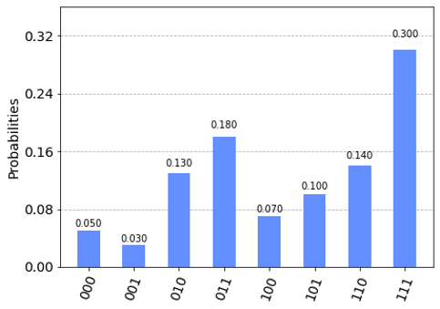
This plot shows a different profile, again stemming from the difference in hardware. Even though Lucy and Aspen-M-1 are both based on superconducting qubits, they have different numbers of qubits and overall topology (i.e., the connectivity between qubits), and were built in labs an ocean apart.
Summary
After completing this tutorial, you have run a circuit to entangle qubits on three different quantum computers through Amazon Braket, coding everything in Qiskit. Check out the additional example notebooks for the qiskit-braket-provider, and consider contributing to one of our open-source Amazon Braket GitHub repos. Have an idea for a new feature or example? You can submit a feature request through a GitHub issue on the repo in question: Amazon Braket Examples or Amazon Braket SDK Python. To connect with the Amazon Braket team on the Qiskit slack workspace, just search for Jordan Sullivan, Zia Mohammad, Poulami Das, or Jon Best.