Using Snowflake to Access and Combine Multiple Datasets Hosted by the Amazon Sustainability Data Initiative

By Aaron Soto, Sustainability Solutions Architect – AWS
By Bosco Albuquerque, Partner Solutions Architect – AWS
By Andries Engelbrecht, Partner Solution Architect – Snowflake

Snowflake

In his book, Greening Through IT, sustainability professor Bill Tomlinson writes that a fundamental challenge with how humans understand and act on environmental issues is that humans are not naturally equipped to operate at the scales of time, space, and complexity that these issues exist.

Throughout history, IT systems have helped humans broaden how we operate across time, space, and complexity. So, while Amazon CEO Andy Jassy states there is no compression algorithm for experience, humans need to utilize advanced IT as compression algorithms to shrink these large environmental issues spanning incomprehensible time, space, and complexity down to human-comprehensible scales.

One piece of IT we are excited about is the zero-cost Amazon Sustainability Data Initiative (ASDI), which seeks to accelerate sustainability research and innovation by minimizing the cost and time required to analyze large sustainability datasets.

These ASDI datasets compress time by storing vast amounts of time-series data, such that users can better understand the past, while also making it possible to predict the future. ASDI datasets compress space by storing data spanning large geographic regions, allowing users to more easily understand the area of the world relevant to their work.

Finally, ASDI datasets compress complexity by aggregating disparate datasets into shared, publicly-accessible locations that are easy to consume using a rapidly-increasing array of Amazon Web Services (AWS) analytics, artificial intelligence (AI), and machine learning (ML) services, as well as prevalent software from AWS Partners.

A growing number of examples exist showing how to use ASDI with AWS-native services. However, we believe it’s important to help customers who use AWS Partner solutions take equal advantage of ASDI datasets in their projects to help us progress towards a more sustainable future.

Snowflake, ASDI Datasets, and Example Use Cases

In this post, we will use Snowflake, a data cloud company, to work with two different ASDI datasets containing climate and air quality data. Snowflake is an AWS Data and Analytics Competency Partner with an enterprise-class SQL engine designed for today’s vast amounts of data.

We’ll use Snowflake to demonstrate how to access ASDI datasets, join them together by date, and ultimately form a merged result. Additionally, we will cover a few best practices from the Sustainability Pillar of the AWS Well-Architected Framework, which was launched at re:Invent 2021.

The first ASDI dataset used in this post is named Global Surface Summary of the Day (GSOD), and contains climate station data for things like temperature, precipitation, and wind. The dataset is published by the National Oceanic and Atmospheric Administration (NOAA).

The second ASDI dataset used is named OpenAQ, and contains air quality readings for pollutants such as 2.5 micron particulate matter, 10 micron particulate matter, ground-level ozone, carbon monoxide, sulfur dioxide, and nitrogen dioxide.

To keep this demo digestible in terms of time, costs, and sustainability, we will use an extra small (XS) Snowflake warehouse—focused on climate data for a single NOAA station in Los Angeles, CA (“USC” Station ID 72287493134) and nearby OpenAQ air quality data within an area of 40X40 km, for a time period of January 2022.

Perhaps you can imagine how analyzing data taken over a larger time span or geographic area could be used by anyone focused on climate contributors to air quality. You could hypothetically select a target air quality pollutant to predict, like ozone, and build a machine learning model that helps accurately indicate how sunlight, temperatures, winds, and other pollutants correlate with ozone concentrations.

Additionally, we encourage you to consider your specific use cases to imagine how you might join in your own data to make intelligent correlations or predictions that could lead to more sustainable outcomes. Generally, climate data informs a wide variety of sustainability efforts and environmental interventions; for example, scientific research to minimize polar ice loss or prevent coral reef bleaching.

Technical Prerequisites

To follow along, you will need the following:

• Snowflake Enterprise Edition account with permission to create storage integrations, ideally in the AWS us-east-1 region or closest available trial region, like us-east-2.

You can subscribe to a Snowflake trial account on AWS Marketplace. In the upper right of the Marketplace listing page, choose Continue to Subscribe, and then choose Accept Terms. You will be redirected to the Snowflake website to begin using the software. To complete your registration, select Set Up Your Account.

• If you’re new to Snowflake, consider completing this Snowflake in 20 minutes tutorial. By the end of the tutorial, you should know how to create required Snowflake objects, including warehouses, databases, and tables for storing and querying data.
  .
• Snowflake worksheet (query editor) and associated access to a warehouse (compute) and database (storage).

Data Characteristics and Sustainable Access Considerations

To begin, we will view the ASDI profile pages for NOAA GSOD and OpenAQ to determine that both of these datasets are located in the North Virginia region (us-east-1). As a sustainability best practice, optimize geographic placement of workloads to use a Snowflake account also located in the same region to minimize data movement.

A great inherent feature of ASDI datasets is that they can be used directly without any need to copy the data. As another sustainability best practice, use shared file systems or object storage to minimize the underlying computing resources needed.

However, sometimes your compute may be in another region or data needs to transformed before querying, which is why we consider data access and storage patterns to minimize overall compute or repeated data transfer needed for these queries.

This post demonstrates how to use Snowflake external stages with external tables directly for the NOAA dataset; as well as how to ultimately create a Snowflake-native materialized view transformed copy of the source data for the OpenAQ dataset.

Create External Stages and External Tables

To get started, log in to your Snowflake account and create a new worksheet linked to your desired warehouse and database. All of the code in this demo can be entered and executed within this worksheet.

Figure 1 below shows a new worksheet and context for role (SYSADMIN), XS-sized warehouse (DEV_WH), database (ASOTO_DB), and schema (PUBLIC).

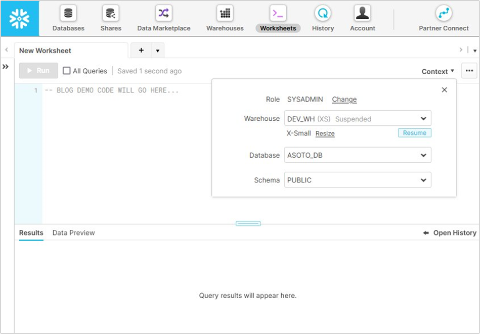
Figure 1 – Context settings in Snowflake worksheets.

We will begin by defining external stages referencing Amazon Simple Storage Service (Amazon S3) bucket locations, which define a pointer to a specific location that can be used to create external tables. These will be defined at the bucket root level, but you can also define stages scoped to a more specific path, if that makes sense for your use case.

-- Create External Stages for each of the two datasets we want to work with...
-- Ext Stage 1: NOAA Global Surface Summary of Day (GSOD)
-- Ext Stage 2: OpenAQ
CREATE OR REPLACE STAGE NOAA_GSOD
URL = 's3://noaa-gsod-pds/';

CREATE OR REPLACE STAGE OPENAQ
URL = 's3://openaq-fetches/';

SHOW STAGES;

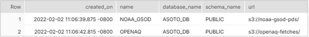
Figure 2 – Result of SHOW STAGES used to verify correct creation of external stages.

With our external stages pointing to these two ASDI dataset buckets, we can create external tables that define any desired subset of the available data. Knowing the characteristics of your source dataset is important, as they are needed to scope your desired table appropriately, as well as supply FILE_FORMAT details.

Our first NOAA dataset for climate data is organized by year + stationIDs and saved as gzipped CSV files with headers and double quote field enclosures, so we will use that in our table definition query.

The second OpenAQ dataset for air quality measurements is organized by date, with each folder containing the entire daily data stored in a series of gzipped newline-delimited JSON files (ndjson). We will define both tables and check our results.

-- Create the NOAA (1) and OpenAQ (2) External Tables as follows...

-- Ext Table 1: NOAAGSOD_2022_LAUSC (LA "USC" station-specific data from 2022)
-- Data Details: https://registry.opendata.aws/noaa-gsod/ (important for FILE_FORMAT)
-- NOTE: The following query should take a few seconds...
CREATE OR REPLACE EXTERNAL TABLE NOAAGSOD_2022_LAUSC
WITH LOCATION = @NOAA_GSOD/2022/
PATTERN = ".*(72287493134).csv"
AUTO_REFRESH = true
FILE_FORMAT = (TYPE=CSV, COMPRESSION=NONE, SKIP_HEADER=1, FIELD_OPTIONALLY_ENCLOSED_BY='"');

-- Ext Table 2: OPENAQ_202201 (all OpenAQ data scoped to 2022-01-**)
-- Data Details: https://registry.opendata.aws/openaq/ (important for FILE_FORMAT)
-- NOTE: Using Snowflake Partitioning by date, to speed up future queries.
-- NOTE: The following query should take a little more than 50 seconds
CREATE OR REPLACE EXTERNAL TABLE OPENAQ_202201(
    AQDATE DATE AS TO_DATE(SUBSTR(metadata$filename, 18, 10), 'YYYY-MM-DD'))
PARTITION BY (AQDATE)     
WITH LOCATION = @OPENAQ/realtime-gzipped/
AUTO_REFRESH = true
FILE_FORMAT = (TYPE=JSON, COMPRESSION=GZIP);

SHOW TABLES;

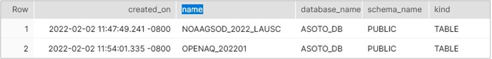
Figure 3 – Result of SHOW TABLES used to verify correct creation of external tables.

We can also quickly query these tables, which consist of records with single columns of the variant data type—a semi-structured data type for hierarchical objects and arrays that are represented as JSON. We can run the following SELECT queries to view results and click on any of the row values to view a JSON representation of the variant value.

-- Quickly explore the data in-place to view/verify structure...
SELECT * FROM NOAAGSOD_2022_LAUSC LIMIT 100;
SELECT * FROM OPENAQ_202201 WHERE AQDATE >= '2022-01-01' AND AQDATE < '2022-02-01' LIMIT 100;

NOAA GSOD Record (CSV)

Selecting from our NOAAGSOD_2022_LAUSC table shows records with clickable variant data type values. Clicking on any row will show the variant’s JSON representation of the source CSV data consisting of enumerated column names and their corresponding values (shown in Figure 4).

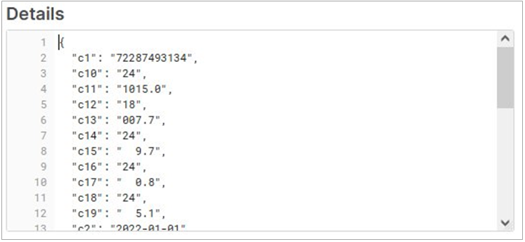
Figure 4 – Details for a single NOAA GSOD row of source CSV data.

OpenAQ Record (JSON)

Selecting from our OPENAQ_202201 table shows records with clickable variant data type values. Clicking on any row will show the variant’s JSON representation matching the source JSON data consisting of the hierarchical name-value pairs according to the source (shown in Figure 5).

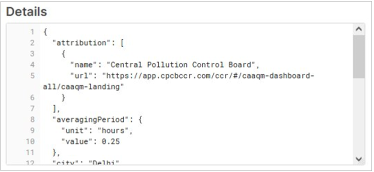
Figure 5 – Details for a single OpenAQ row of source JSON data. 

Working with the NOAA Data Using a Standard, In-Place View

Now, we will prep the NOAA GSOD CSV data as an in-place tabular view containing meaningful column names for the fields relevant to this demo and scoped for downtown Los Angeles in January 2022. Note that knowledge of the CSV file format is necessary in this step.

-- For NOAA GSOD data, we will create a STANDARD view (queries will occur in-place).
-- NOTE: This query took <1sec 
CREATE OR REPLACE VIEW NOAAGSOD_202201_LAUSC_view AS
SELECT DISTINCT
  CAST(value:c1  AS STRING)   AS STATION
, CAST(value:c2  AS DATE)     AS DATE
, CAST(value:c3  AS FLOAT)    AS LATITUDE
, CAST(value:c4  AS FLOAT)    AS LONGITUDE
, CAST(value:c6  AS STRING)   AS NAME
, CAST(value:c7  AS FLOAT)    AS TEMP_AVG
, CAST(value:c23 AS FLOAT)    AS TEMP_MIN
, CAST(value:c21 AS FLOAT)    AS TEMP_MAX
, CAST(value:c17 AS FLOAT)    AS WDSP
, CAST(value:c19 AS FLOAT)    AS MXSPD
, CAST(value:c25 AS FLOAT)    AS PRCP
, CAST(value:c9  AS FLOAT)    AS DEWP
, CAST(value:c15 AS FLOAT)    AS VISIB
FROM    NOAAGSOD_2022_LAUSC
WHERE   DATE >= '2022-01-01' AND DATE < '2022-02-01';

-- Quickly check how this looks...
SELECT * FROM NOAAGSOD_202201_LAUSC_VIEW LIMIT 100;

If you query your new view, you’ll get 31 records returned—one for each day in January, the first 10 shown in Figure 6 below. If we were looking at a larger time span or a wider geographic selection of stations, we could perform in-place queries over vast amounts of time and space to understand average temperatures over decades, for example.

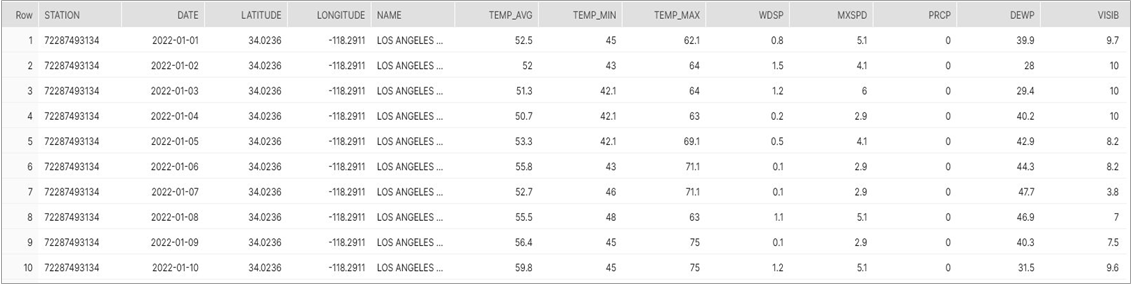
Figure 6 – Results from the SELECT query showing the first 10 of 31 rows returned.

Working with the OpenAQ Data Using a Materialized View

Next, let’s prep the OpenAQ JSON data using a materialized view. This will create a Snowflake-native copy of our relevant subset of the data to allow for more efficient querying (compute) as we perform additional transformations.

As part of our transformations, we will use Snowflake’s PIVOT construct to turn rows based on individual air quality measurements into a tabular view based on the date, with columns containing air quality averages. This column-based structure is similar to our climate data, so that the two datasets can be JOINed together for a merged result.

The six relevant OpenAQ parameters in this data are carbon monoxide (CO), nitrogen dioxide (NO₂), ozone (O₃), sulfur dioxide (SO₂), particulate matter <= 2.5 microns (PM2.5), and particulate matter <=10 microns (PM10).

-- For larger operations we will dynamically scale the Snowflake warehouse for faster execution
-- This is a MATERIALIZED view (queries will occur over our optimized data copy).
-- Additional sourceType + mobile filter to get fixed, reference grade data only.
-- Additional Lat/Lng filter to get data around Los Angeles, CA, US (~40km x ~40km box centered around downtown LA)
-- NOTE: This query took ~5:00mins on an XS warehouse...
CREATE OR REPLACE MATERIALIZED VIEW OPENAQ_202201_LA_MVIEW AS
SELECT DISTINCT
  CAST(value:date:utc              AS DATETIME) AS date_utc
, CAST(value:date:local            AS DATETIME) AS date_local
, CAST(value:sourceName            AS STRING)   AS source_name
, CAST(value:sourceType            AS STRING)   AS source_type
, CAST(value:parameter             AS STRING)   AS measurement_parameter
, CAST(value:unit                  AS STRING)   AS measurement_unit
, CAST(value:value                 AS FLOAT)    AS measurement_value
, CAST(value:mobile                AS BOOLEAN)  AS is_mobile
, CAST(value:coordinates:latitude  AS FLOAT)    AS coords_latitude
, CAST(value:coordinates:longitude AS FLOAT)    AS coords_longitude
, CAST(value:country               AS STRING)   AS loc_country
, CAST(value:city                  AS STRING)   AS loc_city
, CAST(value:location              AS STRING)   AS loc_location
, CAST(value:averagingPeriod:unit  AS STRING)   AS averagingperiod_unit
, CAST(value:averagingPeriod:value AS FLOAT)    AS averagingperiod_value
, CAST(value:attribution           AS VARIANT)  AS attribution
, AQDATE
FROM    OPENAQ_202201
WHERE   AQDATE >= '2022-01-01' AND AQDATE < '2022-02-01'
        AND value:date:local >= '2022-01-01' AND value:date:local < '2022-02-01'
        AND value:sourceType IN ( 'government' )
        AND CAST(value:mobile AS BOOLEAN) = false
        AND CAST(value:coordinates:latitude  AS FLOAT) >=   33.8707 AND CAST(value:coordinates:latitude  AS FLOAT) <=   34.2315
        AND CAST(value:coordinates:longitude AS FLOAT) >= -118.4157 AND CAST(value:coordinates:longitude AS FLOAT) <= -118.0549;
-- Quickly check how this looks...
SELECT * FROM OPENAQ_202201_LA_mview ORDER BY date_local, measurement_parameter, loc_location  LIMIT 100;

This new materialized view shows data from four nearby locations—including Compton, Los Angeles, Pasadena, and Pico Rivera—sampled hourly for any of the six air quality parameters. This means we have up to 576 records for each day. (4 x 24 x 6; and in actuality, the records for a day are less since some stations may not report all parameters or may have missing hourly samples.)

For this demo, we want an aggregated daily average of the six available air quality parameters so we can join those alongside our daily summarized climate data from NOAA. To do this, let’s continue prep work over this materialized view.

-- Get a view of daily averages per parameter...
CREATE OR REPLACE VIEW OPENAQ_202201_LADailyAvgs_view AS
SELECT to_date(date_local) AS date_local, measurement_parameter, AVG(measurement_value) AS measurement_value_avg
FROM   OPENAQ_202201_LA_mview
GROUP BY to_date(date_local), measurement_parameter
ORDER BY to_date(date_local), measurement_parameter;

--> Let's take a look, we should have 186 records (31 days * 6 averaged measurements/day)
SELECT * FROM OPENAQ_202201_LADailyAvgs_view ORDER BY date_local, measurement_parameter LIMIT 200;

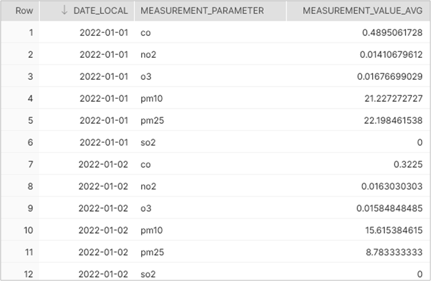
Figure 7 – Averages of row-based air quality with six measurements per date.

Let’s PIVOT this row-based data into column-based data, so that we have one row per date:

-- Since OpenAQ data has rows for each parameter, we'd like a pivoted view of parameters as columns for each data...
CREATE OR REPLACE VIEW OPENAQ_202201_LADailyAvgsPivoted_view AS
SELECT * 
FROM OPENAQ_202201_LADailyAvgs_view
     PIVOT(AVG(measurement_value_avg) FOR measurement_parameter IN ('co', 'no2', 'o3', 'pm10', 'pm25', 'so2'))
       AS p (date_local, co_avg_ppm, no2_avg_ppm, o3_avg_ppm, pm10_avg_ugm, pm25_avg_ugm, so2_avg_ppm)
ORDER BY date_local;

SELECT * FROM OPENAQ_202201_LADailyAvgsPivoted_view ORDER BY date_local LIMIT 31;

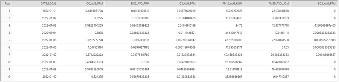
Figure 8 – Screenshot of pivoted results with one row per date like our climate data.

Now that we have climate data from NOAA and air quality data from OpenAQ, we can perform a JOIN to get to our final desired result of a merged dataset that can theoretically be used for the types of correlations or predictions explored earlier.

-- Finally, JOIN the NOAA GSOD data with the averaged+pivoted OpenAQ dataset into a single view by date...
CREATE OR REPLACE VIEW JoinedClimateAndAQ_LosAngeles_DailyAvgs_view AS
SELECT  noaa.*,
        aq.co_avg_ppm, aq.no2_avg_ppm, aq.o3_avg_ppm, aq.pm10_avg_ugm, aq.pm25_avg_ugm, aq.so2_avg_ppm
FROM    NOAAGSOD_202201_LAUSC_view noaa
        LEFT OUTER JOIN OPENAQ_202201_LADailyAvgsPivoted_view aq ON noaa.DATE = aq.date_local
ORDER BY noaa.DATE;

SELECT * FROM JoinedClimateAndAQ_LosAngeles_DailyAvgs_view ORDER BY DATE;

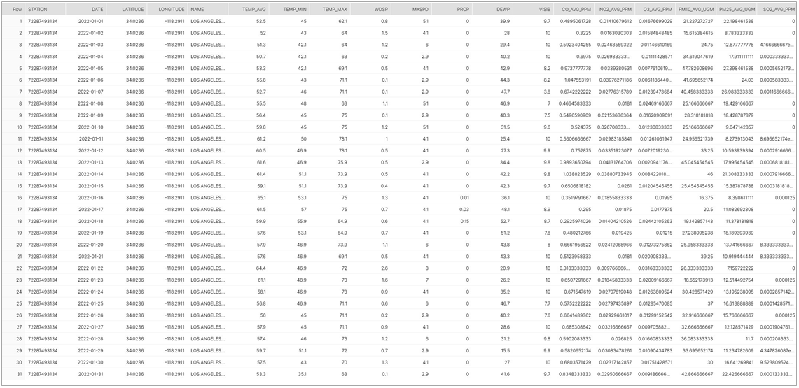
Figure 9 – Final SELECT query result showing JOINed NOAA climate and OpenAQ values by date.

Summary

Many organizations and research scientists use data every day to help solve challenges or work towards a more environmentally sustainable future.

The Amazon Sustainability Data Initiative (ASDI) offers access to vast amounts of data that can help people make progress towards sustainability challenges by compressing time, space, and complexity by more easily consuming this data in various analytics tools.

AWS-native services and AWS Partner solutions are great examples of tools that can process this data. In this post, we explored how to use Snowflake to create both in-place and materialized views that can be queried, transformed, and joined together into new results.

While this post used a small subset of data, you can see how these tools could query vast amounts of merged climate and air quality data or use the merged result as input into a machine learning model that could predict air quality outcomes based on climate data.

To learn more, we recommend you review these additional resources:

• Amazon Sustainability Data Initiative (ASDI)
  • NOAA Global Surface Summary of Day (global surface climate data)
  • OpenAQ (global air quality data)
• Snowflake Docs
  • Create Stage (including external stages for Amazon S3 buckets)
  • Create External Table
  • Create View
  • Create Materialized View
  • PIVOT Construct

.

.

Snowflake – AWS Partner Spotlight

Snowflake is an AWS Competency Partner that has reinvented the data warehouse, building a new enterprise-class SQL data warehouse designed from the ground up for the cloud and today’s data.

Contact Snowflake | Partner Overview | AWS Marketplace

*Already worked with Snowflake? Rate the Partner

*To review an AWS Partner, you must be a customer that has worked with them directly on a project.