AWS Big Data Blog
Estimate Amazon EC2 Spot Instance cost savings with AWS Glue DataBrew, AWS Glue, and Amazon QuickSight
AWS provides many ways to optimize your workloads and save on costs. For example, services like AWS Cost Explorer and AWS Trusted Advisor provide cost savings recommendations to help you optimize your AWS environments. However, you may also want to estimate cost savings when comparing Amazon Elastic Compute Cloud (Amazon EC2) Spot to On-Demand Instances.
In this post, I show you how to estimate savings with Spot Instances based on your organization’s historical On-Demand usage. Keep in mind that cost savings differ based on instance types, Availability Zones, presence of Savings Plans, and other variables.
Additionally, I show you how to set up and automate data processing with AWS CloudFormation and AWS Glue DataBrew via the AWS Management Console so that you can easily get these results without needing deep knowledge in data engineering and coding.
Overview
EC2 Spot Instances are spare compute capacity in the AWS Cloud available to you at up to 90% savings compared to On-Demand Instances. The savings are significant because Spot Instances can be interupted by Amazon EC2 with 2 minutes of notification. However, you can architect your environment to build resilient workloads. For more information, see Best practices for handling EC2 Spot Instance interruptions.
AWS Glue is a serverless data integration service that makes it easy to transform, prepare, and analyze data for your analytics and machine learning workloads. You can run your Glue jobs as new data arrives. For example, you can use an AWS Lambda function to trigger your Glue jobs to run when new data becomes available in Amazon S3.
AWS Glue DataBrew is a new visual data preparation tool that makes it easy for data analysts and data scientists to clean and normalize data to prepare it for analytics and machine learning (ML). We use DataBrew to eliminate the need to write any code for transforming AWS Cost and Usage Reports (AWS CUR). Even if you don’t have many data engineers in your organization, you easily transform, automate, and prepare data sets for analysis.
Cost and Usage Reports contain the most comprehensive set of cost and usage data available. We use a monthly CUR file as the data source to view historical Amazon EC2 On-Demand usage and compare that to what could have been saved if we had used Spot. We then visualize these results with Amazon Quicksight, a scalable, serverless, embeddable, ML-powered business intelligence (BI) service built for the cloud. QuickSight lets you easily create and publish interactive BI dashboards that include ML-powered insights.
The following architectural diagram illustrates what we cover in this post:

You start by using the CUR as the data source for historical usage. You then use a DataBrew recipe to transform the data and retrieve only Amazon EC2 On-Demand usage. When the transformation is complete, an AWS Lambda function triggers an AWS Glue Python shell job to retrieve the historical Spot prices for a particular EC2 instance configuration. Lastly, you use QuickSight to visualize the results.
Deploy AWS CloudFormation Template
We deploy a CloudFormation template to provision resources that include an Amazon Simple Storage Service (Amazon S3) bucket, an AWS Glue Python shell job, a DataBrew recipe, and the necessary AWS Identify and Access Management (IAM) roles.
The DataBrew recipe filters the CUR file to only include EC2 On-Demand Instance usage for a reporting month. It then extracts information needed to feed into the AWS Glue Python shell job to get historical Spot price data (for example, the Availability Zone, the instance type, or the operating system).
The AWS Glue Python shell job takes the output from DataBrew and uses the describe-spot-price-history API to retrieve historical Spot prices for that particular instance configuration. It gathers the minimum, maximum, and average prices for the usage time period because the price can vary. We use an AWS Glue Python shell job for retrieving the historical Spot prices to avoid timing out, which may occur if we use Lambda.
To deploy your resources, complete the following steps:
- Deploy the CloudFormation stack in your desired Region (for this post, we use
us-east-1; check the AWS Regional Services List).


- For Stack name, enter a name.
- Choose Next.
- Proceed through the steps and acknowledge that AWS CloudFormation might create IAM resources with custom names.

- Choose Create stack.
Data Transformation with AWS Glue DataBrew
You can use the CUR to understand your service usage costs. After you set up the CUR, AWS delivers cost and usage data to an S3 bucket and generates hourly, daily, or monthly usage reports. In this case, we use a daily CUR as the data source for a particular month.
We need to create a dataset in DataBrew that points to a month’s usage. (You must select monthly usage within the past 3 months because the DescribeSpotPriceHistory API gathers price data up to the past 90 days).
- On the DataBrew console, connect to a new dataset by providing a name and specifying the source path in Amazon S3.

- When the dataset connection is complete, choose Create project with this dataset.

The CloudFormation template creates a working version of a DataBrew recipe. A recipe is a collection of data transformation steps. You can create your own, edit them in a DataBrew project, or publish them as a stand-alone entity.
- For Project name, enter a name.
- For Attached recipe, choose Edit existing recipe.
- Choose the recipe the CloudFormation template created. This can be found under Attached recipe, and then by selecting Edit existing recipe.
- Under Select a dataset, select My datasets.
- Choose your dataset.

- Under Sampling, you can specify the type and size of the sample. For this post, I use a random sample size of 500.
- In the Permissions section, you can authorize DataBrew to create a role on your behalf with the necessary permissions to access the dataset. You can also create a custom role if desired.

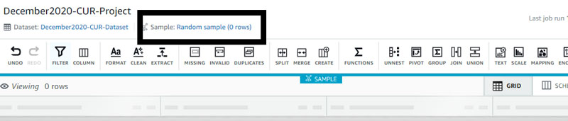
After you create the project, DataBrew imports the recipe and validates the steps. The recipe steps are documented in the Recipe pane. You can see the changes when the import is complete.
To quickly summarize, the recipe renames key columns for the AWS Glue Python shell job, splits columns on a delimiter from the UsageStart and UsageEnd columns, and filters the data to select only On-Demand Instance line items.

If you don’t see any data, you can change the sample size and sample selection on the top menu.
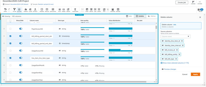
Feel free to delete columns that you don’t want to include in the final analysis. However, you must keep the columns that were renamed by the recipe, otherwise the AWS Glue job encounters an error.
An easy way to delete unwanted columns is to select the Schema view and select all the columns you want to delete while deselecting the columns you want to keep (the columns you want to keep don’t have the underscore character as a column header).
- Make any desired changes to the columns and choose Apply.
You may want to keep certain colums, as well. For instance, you may want to include tag columns to keep On-Demand Instances with a particular tag (such as ‘dev‘ or ‘test‘). You may want to do this to run the analyses on workloads where the savings from Spot Instances are greater, or for a particular workload.
After you include the rows and columns you want in the final output, we’re ready for DataBrew to transform the data and subsequently trigger the AWS Glue job. Select Create job at the top-right corner of the page.
- Choose Create job.
- Name your job and specify the output location as the S3 bucket the CloudFormation stack created.
This bucket must be the location to successfully trigger the AWS Glue job.
- Under Additional Configuration, select Replace output files for each job run.

- Choose the IAM role created previously by DataBrew or your own custom role.
- Choose Create and run job.
The job takes a few minutes to run. You can check on the job status on the Jobs page of the console.

DataBrew outputs the resulting CSV into the S3 bucket folder created by the CloudFormation template. The PutObject event triggers the Lambda function to start an AWS Glue job to get historical Spot prices.
When the job is complete, check the Amazon S3 bucket and to see a file uploaded with the Spot price results. The job appended three columns: the average, minimum, and maximum Spot prices gathered for the usage start and end times.
Download this CSV to your local machine. We upload this file as a dataset in QuickSight for visualization. We can also set up an Athena table by crawling the data for QuickSight to directly access the data set. We avoid that extra step by uploading the dataset to QuickSight instead.
Visualizing in QuickSight
QuickSight is a cloud-based BI service that you can use to quickly deliver insights to relevent parties within your organization. We use QuickSight to compare On-Demand costs to Spot costs.
To get started with QuickSight, see Tutorial: Create A Multivisual Analysis and a Dashboard Using Sample Data. We upload the CSV file as a dataset to populate our analysis.

Set up an analysis
To configure your analysis, complete the following steps:
- On the QuickSight start page, choose New analysis.
- Select New dataset.
- Choose Upload a file.

- Choose the CSV output file DataBrew created.
- Choose Next.
The CSV files auto-ingest to SPICE, which helps boost performance.
- Choose Visualize.
We can estimate cost savings now that we have the average, minimum, and maximum Spot prices. For example, we can create a calculated field with the following steps:
- On the Add menu, choose Add calculated field.

- Enter a name for the calculated field (for example,
EstimatedAvgSavings ($)). - Enter a formula that calculates the difference between the
OnDemandPriceandAverageSpotPrice, multiplied byUsageQuantity. - Choose Save.

This field shows what you could have saved in actual dollars, if you used Spot instead of On-Demand Instances.
Visualizing Savings
Now that you have a calculated field, you can combine this field with other columns for better insight into cost savings.
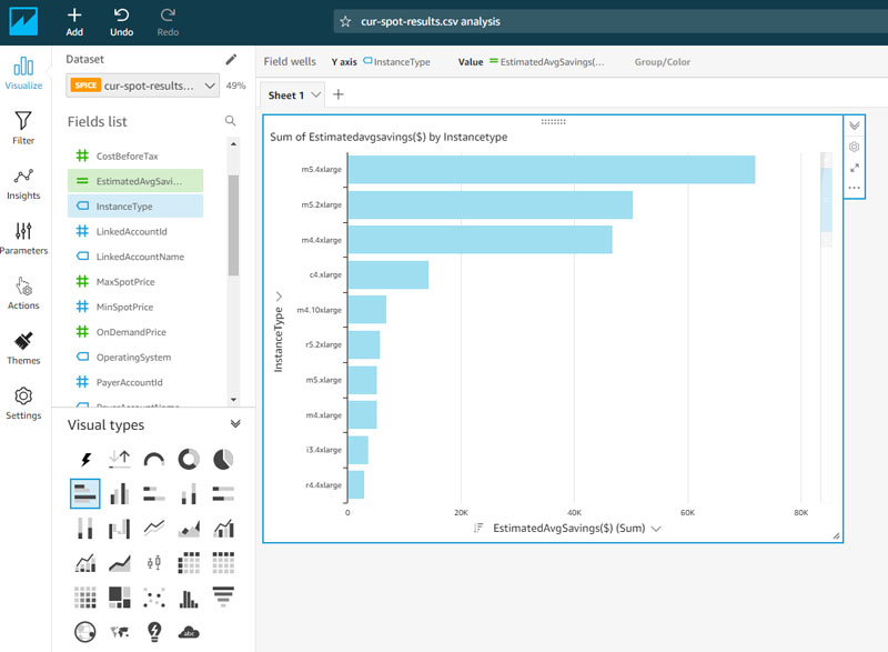
- Under Visual types, choose the horizontal bar chart.
- For Y axis, choose InstanceType.
- For Value, choose the calculated field you created (
EstimatedAvgSavings($)).
QuickSight automatically generates the visual, sorting the top potential savings by instance type. You can scroll down within the visual frame to see savings for additional instance types.
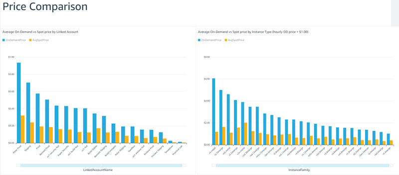
You can create other fields such as taking a percentage of savings (rather than the monetary difference), compare savings by Region or Availability Zone, and see savings by linked account.
Because the CUR includes tagged resources, you can do the same exercise for tagged EC2 instances as well, for example filtering only on instances that are tagged with environment values as dev or test. You can be creative to focus on workloads that make the most sense for your organization.


Conclusion
In this post we used DataBrew to transform CUR data for an AWS Glue job to get historical Spot prices for usage data. We then visualized these results in QuickSight for better insight into how much savings we could realize by moving some On-Demand workloads to Spot.
There are many more ways to view and analyze your CUR data to find opportunities to optimize your AWS environment.
About the Author
 Peter Chung is a Solutions Architect for AWS, and is passionate about helping customers uncover insights from their data. He has been building solutions to help organizations make data-driven decisions in both the public and private sectors. He holds all AWS certifications as well as two GCP certifications. He enjoys coffee, cooking, staying active, and spending time with his family.