How Imperva uses Amazon Athena for machine learning botnets detection

This is a guest post by Ori Nakar, Principal Engineer at Imperva. In their own words, “Imperva is a large cyber security company and an AWS Partner Network (APN) Advanced Technology Partner, who protects web applications and data assets. Imperva protects over 6,200 enterprises worldwide and many of them use Imperva Web Application Firewall (WAF) solutions to secure their public websites and other web assets.”

In this post, we explain how Imperva used Amazon Athena, Amazon SageMaker, and Amazon QuickSight to develop a machine learning (ML) clustering algorithm that can efficiently detect botnets attacking your infrastructure.

Athena is an interactive query service that makes it easy to analyze data in Amazon Simple Storage Service (Amazon S3) using standard SQL. Athena is serverless, easy to use, and makes it easy for anyone with SQL skills to quickly analyze large-scale datasets in multiple Regions.

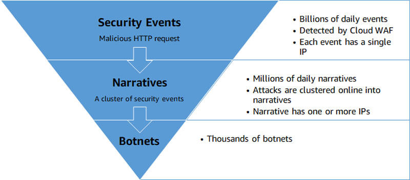
Imperva Cloud WAF protects hundreds of thousands of websites and blocks billions of security events every day. Security events are correlated online into security narratives, and an innovative offline process enables you to detect botnets. Events, narratives, and many other security data types are stored in Imperva’s Threat Research multi-Region data lake.

Botnets and data flow

Botnets are internet connected devices that perform repetitive tasks, such as Distributed Denial of Service (DDoS). In many cases, these consumer devices are infected with malicious malware that is controlled by an external entity, often without the owner’s knowledge. Imperva botnet detection allows you to enhance your website’s security and get detailed information on botnet attacks and come up with ways to mitigate their impact.

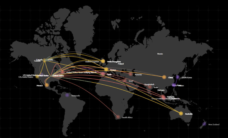
The following is a visualization of a botnets attack map. Each botnet can be composed of tens to thousands of IPs, one or more source location, and one or more target locations, performing an attack such as DDoS, vulnerability scanning, and others.

The following diagram illustrates Imperva’s flow to detect botnets.

The remainder of this post dives into the process of developing the botnet detection capability and describes the AWS services Imperva uses to enable and accelerate it.

Botnet detection development process

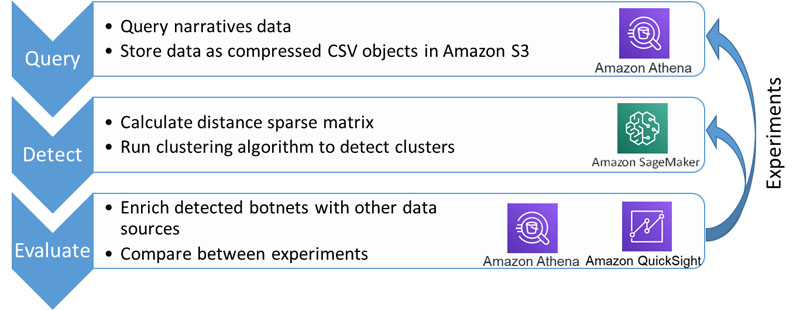
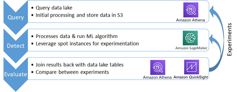
Imperva’s development process has three main steps: query, detect and evaluate. The following diagram summarizes these steps.

Query

Imperva stores the narrative data in Imperva’s Threat Research data lake. Data is continuously added as objects to Amazon S3 and stored in multiple Regions due to regulation and data locality requirements. For more information about querying data stored in multiple Regions using Athena, see Running SQL on Amazon Athena to Analyze Big Data Quickly and Across Regions.

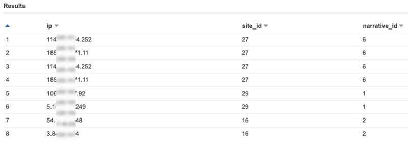
One of the tables in the data lake is the narratives tables, which has the following columns.

Column	Description
`narrative_id`	ID of a detected narrative.
`ip`	Each narrative has one or more IPs.
`site_id`	ID of the attacked site. Narrative has a single attacked site.

The following screenshot is a sample of the data being queried.

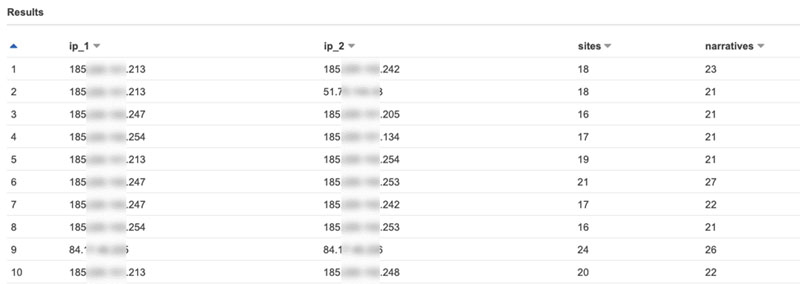
Finding correlations between attacking IPs of the same website generates our initial dataset, which allows us to hone in on those that are botnets. The following query in Athena generates that initial list.

The query first finds narratives and sites per IP, and stores those in arrays. Next, the query finds all the pairs using a SELF JOIN (L for left, R for right). For each IP pair, it calculates the number of narratives and number of attacked sites. Then it filters on pairs with one common narrative. See the following code:

-------------------- STEP 1 --------------------
WITH nar_ips AS (
 SELECT ip, ARRAY_AGG(narrativ_id) AS ids,
        ARRAY_AGG(site_id) AS sites
 FROM narratives
 GROUP BY 1) 
-------------------- STEP 2 --------------------
SELECT l.ip AS ip_1, r.ip AS ip_2,
  CARDINALITY(ARRAY_INTERSECT(l.ids, r.ids)) AS narratives,
  CARDINALITY(ARRAY_INTERSECT(l.sites, r.sites)) AS sites
FROM nar_ips AS l INNER JOIN nar_ips AS r ON
  l.ip < r.ip
  AND ARRAYS_OVERLAP(l.ids, r.ids)

The following screenshot shows a query result of IP pairs that attacked the same websites and the number of attacks that they performed together.

Imperva uses Create Table as Select (CTAS) to store the query results in Amazon S3 using a CSV file format that the SageMaker training job uses in the next step. Use the following query:

CREATE TABLE [temp_table_name]
WITH (format='TEXTFILE',
  bucketed_by=ARRAY['ip_1'], bucket_count=5,
  external_location='s3://my-bucket/my-temp-location',
  field_delimiter = ',') AS [SQL]

The TEXTFILE format saves the data compressed as gzip, and the bucketing information controls the number of objects and therefore their sizes. Athena CTAS supports multiple types of data formats, and it’s recommended to evaluate which file format is best suited for your use case.

The following screenshot shows objects created in the S3 data lake by Athena.

Detect: Botnets clustering

The next step in Imperva’s process is to cluster the IP pairs from the previous step into botnets. This includes steps for input, model training and output.

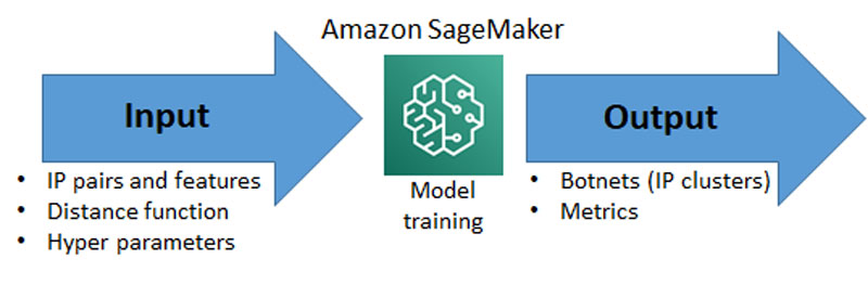
Input

The first step is to calculate the distance between each IP pair in a narrative. This process raises a couple of options. The first is if you use Athena with either the included analytic functions such as cosine_similarity, or develop a custom UDF to perform the calculation. For Imperva’s needs, we decided to use SageMaker and implement the distance calculation using Python.

For other implementations, you should experiment with your data and decide which big data processing method to use. The following diagram shows some of the characteristics of each method.

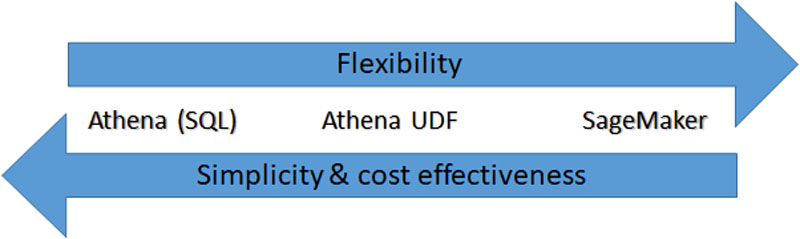
Each language has different capabilities. For example, Java and Python are much more flexible than SQL, but makes the pipeline more complex in terms of development and maintenance. The volume of data consumed and processed by SageMaker directly impacts the time it takes to complete the model training.

Model training and output

We use the SageMaker Python SDK to create a training job, which is used for the model training. The jobs are created and monitored using simple Python code. When running the training job, you can choose which remote instance type best fits the needs of the job, and use Amazon Elastic Compute Cloud (Amazon EC2) Spot Instances to save costs. Imperva used the Python Scikit-learn base image, which includes all libraries required, and more libraries can be installed if needed. Logs from the remote instance are captured for monitoring, and when the job is complete, the output is saved to Amazon S3. See the following code:

from sagemaker.sklearn import SKLearn

estimator = SKLearn(entry_point="my_script.py",
                    use_spot_instances=True,
                    hyperparameters={"epsilon": 0.1,
                                     "min_samples": 10},
                    instance_type="ml.m4.xlarge")
estimator.fit(inputs={"train": "s3://my_bucket/my_folder"})

The following code is the details of the script running in the remote instance that was launched.

The distance function gets a list of features and returns a distance between 0–1:

def distance(narratives: int, sites: int) -> float:
   return  1 - (1 / sites) -
                (1 / narratives)

SageMaker copies the data from Amazon S3 and runs the calculation of distance based on all IP pairs. The following code goes over the files and records:

distances_arr = []

for file_name in file_names:
   df = pd.read_csv(file_name, header=None, chunksize=100_000,
       names=["ip_1", "ip_2", "sites", "narratives"])
   for _, row in df.iterrows():
       distances_arr.append(distance(row["sites"],
                                     row["narratives"]))

The output of that calculation is transformed into a sparse distance matrix, which is fed into a DBSCAN algorithm and detects clusters. DBSCAN is one of the most common clustering algorithms. DBSCAN runs on a given set of points; it groups together points that are closely packed together. See the following code:

model = DBSCAN(eps=0.1, min_samples=10, metric="precomputed")
result = model.fit_predict(dist_mat)

When the clustering results are ready, SageMaker writes the results to Amazon S3. The table is created by copying the output of SageMaker to a new table partition in Amazon S3.

The results are IP clusters, and a working pipeline is established. The following screenshot shows an example of the clustering algorithm results.

The pipeline allows for the evaluation and experimentation phase to begin. This is often the more time-consuming phase to help ensure optimal results are achieved.

Evaluate: Run various experiments and compare between them

The IP clusters (which Imperva refers to as botnets) that were found are written back to a dedicated table in the data lake.

You can run the botnet detection process with different parameters within SageMaker. The following are some examples of parameters that you can alter:

Adjust query parameters such as IP hits, sites hits, and more
Change the distance function being used
Adjust hyperparameters such as DBScan epsilon and minimum samples
Change the clustering algorithm being used (for example, OPTICS)

After you complete several experiments, the following step is to compare them. Imperva accomplishes this by using Athena to query the results for a set of experiments and joining the detected botnet IP data with various additional tables in the data lake.

The following example code walks through joining the detected botnet IP data with newer narratives data:

WITH narratives_ips AS (
  SELECT experiment, botnet, ip, narrarive_id
  FROM botnets INNER JOIN narratives USING (validation_day, ip))
SELECT experiment, botnet, narrarive_id, COUNT() AS ips
GROUP BY 1,2,3

For each detected botnet, Imperva finds the relevant narratives and checks if those IPs continue to jointly attack as a group.

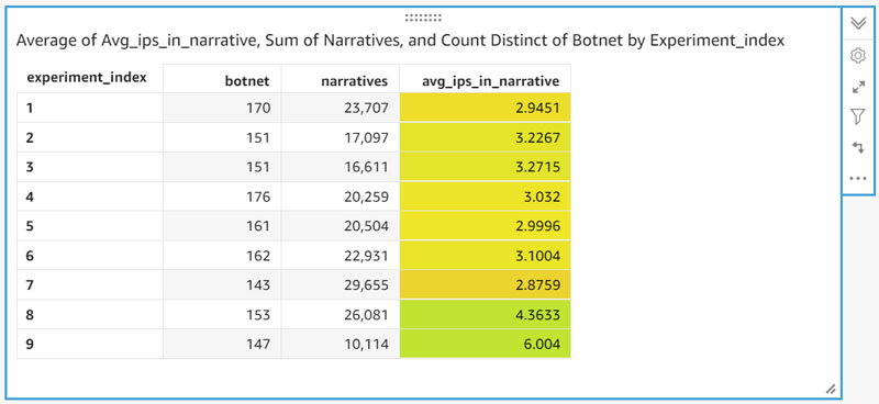
Visualizing results from multiple experiments allows you to quickly glean their level effectiveness. Imperva uses QuickSight connected to Athena to query and visualize the experiments table. In the following analysis example, for each experiment, the following information is reviewed:

Number of botnets
Total number of narratives
Average number of IPs in a narrative—this means that the same IPs continued to attack as a group, as predicted

The data is visualized using a pivot table in QuickSight, and additional conditional formatting allows for an easy comparison between experiments.

To further analyze the results, it was hypothesized that the number of tools used by the botnet might provide additional insights. These tools could be custom-built code or common libraries such as PhantonJS used in malicious ways.

The tool information is added to the pivot table, with the ability to drill down to each experiment to view how many tools were used by each botnet.

The tool hypothesis is just one example of the analyses available. It’s also possible to drill down further and view the sum of narratives by tool as a donut chart. This visualization can help you quickly see the distribution of tools in a specific experiment. You can perform such analysis on any other field, table, or data source.

Imperva uses this method to analyze, compare, and fine-tune experiments in order to improve results.

Summary

Thousands of customers use the Imperva Web Application Firewall to defend their applications from hacking and denial of service attacks. The most common source of these attacks are botnets, comprised of a large network of computers across the internet. For Imperva to improve our ability to identify, isolate, and stop these attacks, we developed a simple pipeline that allows us to quickly collect and store network traffic in Amazon S3 and analyze it using Athena to identify patterns. We used SageMaker to quickly experiment with different clustering and ML algorithms that help detect patterns in botnet activity.

You can generalize this flow to other ML development pipelines, and use any part of it in a model development process. The following diagram illustrates the generalized process.

Running many experiments quickly and easily helps achieve business objectives faster. Running experiments on large volumes of data often requires a lot of time and can be rather expensive. An AWS-based processing pipeline eliminates these challenges by utilizing various AWS services:

Athena to quickly and cost-effectively analyze large amounts of data
SageMaker to experiment with different ML algorithms in a scalable and cost-effective manner
QuickSight to visualize and dive deep into the data in order to extract critical insights that help you fine-tune your ML models

This blog post is based on a demo at re:Invent 2020 by the authors. You can watch that presentation on YouTube.

About the Authors

Ori Nakar is Principal Engineer at Imperva’s Threat Research Group. His main interests are WEB application and database security, data science, and big data infrastructure.

Yonatan Dolan is a Business Development Manager at Amazon Web Services. He is located in Israel and helps customers harness AWS analytical services to leverage data, gain insights, and derive value.