AWS Database Blog
Building a knowledge graph with topic networks in Amazon Neptune
This is a guest blog post by By Edward Brown, Head of AI Projects, Eduardo Piairo, Architect, Marcia Oliveira, Lead Data Scientist, and Jack Hampson, CEO at Deeper Insights.
We originally developed our Amazon Neptune-based knowledge graph to extract knowledge from a large textual dataset using high-level semantic queries. This resource would serve as the backend to a simplified, visual web-based knowledge extraction service. Given the sheer scale of the project—the amount of textual data, plus the overhead of the semantic data with which it was enriched—a robust, scalable graph database infrastructure was essential.
In this post, we explain how we used Amazon’s graph database service, Neptune, along with complementing Amazon technologies, to solve this problem. Some of our more recent projects have required that we build knowledge graphs of this sort from different datasets. So as we proceed with our explanation, we use these as examples. But first we should explain why we decided on a knowledge graph approach for these projects in the first place.
Our first dataset consists of medical papers describing research on COVID-19. During the height of the pandemic, researchers and clinicians were struggling with over 4,000 papers on the subject released every week and needed to onboard the latest information and best practices in as short a time as possible. To do this, we wanted to allow users to create their own views on the data—custom topics or themes—to which they could then subscribe via email updates. New and interesting facts within those themes that appear as new papers are added to our corpus arrive as alerts to the user’s inbox. Allowing a user to design these themes required an interactive knowledge extraction service.
This eventually became the Covid Insights Platform. The platform uses a Neptune-based knowledge graph and topic network that takes over 128,000 research papers, connects key concepts within the data, and visually represents these themes on the front end.
Our second use case originated with a client who wanted to mine articles discussing employment and occupational trends to yield competitor intelligence. This also required that the data be queried by the client at a broad, conceptual level, where those queries understand domain concepts like companies, occupational roles, skill sets, and more. Therefore, a knowledge graph was a good fit for this project.
We think this article will be interesting to NLP specialists, data scientists, and developers alike, because it covers a range of disciplines, including network sciences, knowledge graph development, and deployment using the latest knowledge graph services from AWS.
Datasets and resources
We used the following raw textual datasets in these projects:
- CORD-19 – CORD-19 is a publicly available resource of over 167,000 scholarly articles, including over 79,000 with full text, about COVID-19, SARS-CoV-2, and related coronaviruses.
- Client Occupational Data – A private national dataset consisting of articles pertaining to employment and occupational trends and issues. Used for mining competitor intelligence.
To provide our knowledge graphs with structure relevant to each domain, we used the following resources:
- Unified Medical Language System (UMLS) – The UMLS integrates and distributes key terminology, classification and coding standards, and associated resources to promote creating effective and interoperable biomedical information systems and services, including electronic health records.
- Occupational Information Network (O*NET) – The O*NET is a free online database that contains hundreds of occupational definitions to help students, job seekers, businesses, and workforce development professionals understand today’s world of work in the US.
Adding knowledge to the graph
In this section, we outline our practical approach to creating knowledge graphs on Neptune, including the technical details and libraries and models used.
To create a knowledge graph from text, the text needs be given some sort of structure that maps the text onto the primitive concepts of a graph like vertices and edges. A simple way to do this is to treat each document as a vertex, and connect it via a has_text edge to a Text vertex that contains the Document content in its string property. But obviously this sort of structure is much too crude for knowledge extraction—all graph and no knowledge. If we want our graph to be suitable for querying to obtain useful knowledge, we have to provide it with a much richer structure.
Ultimately, we decided to add the relevant structure—and therefore the relevant knowledge—using a number of complementary approaches that we detail in the following sections, namely the domain ontology approach, the generic semantic approach, and the topic network approach.
Domain ontology knowledge
This approach involves selecting resources relevant to the dataset (in our case, UMLS for biomedical text or O*NET for documents pertaining to occupational trends) and using those to identify the concepts in the text. From there, we link back to a knowledge base providing additional information about those concepts, thereby providing a background taxonomical structure according to which those concepts interrelate.
That all sounds a bit abstract, granted, but can be clarified with some basic examples.
Imagine we find the following sentence in a document:
Semiconductor manufacturer Acme hired 1,000 new materials engineers last month.
This text contains a number of concepts (called entities) that appear in our relevant ontology (O*NET), namely the field of semiconductor manufacturers, the concept of staff expansion described by “hired,” and the occupational role materials engineer. After we align these concepts to our ontology, we get access to a huge amount of background information contained in its underlying knowledge base. For example, we know that the sentence mentions not only an occupational role with a SOC code of 17-2131.00, but that this role requires critical thinking, knowledge of math and chemistry, experience with software like MATLAB and AutoCAD, and more.
In the biomedical context, on the other hand, the text “SARS-coronavirus,” “SARS virus,” and “severe acute respiratory syndrome virus” are no longer just three different, meaningless strings, but a single concept—Human Coronavirus with a Concept ID of C1175743—and therefore a type of RNA virus, something that could be treated by a vaccine, and so on.
In terms of implementation, we parsed both contexts—biomedical and occupational—in Python using the spaCy NLP library. For the biomedical corpus, we used a pretrained spaCy pipeline, SciSpacy, released by Allen NLP. The pipeline consists of tokenizers, syntactic parsers, and named entity recognizers retrained on biomedical corpora, along with named entity linkers to map entities back to their UMLS concept IDs. These resources turned out to be really useful because they saved a significant amount of work. For the occupational corpora, on the other hand, we weren’t quite as lucky. Ultimately, we needed to develop our own pipeline containing named entity recognizers trained on the dataset and write our own named entity linker to map those entities to their corresponding O*NET SOC codes.
In any event, hopefully it’s now clear that aligning text to domain-specific resources radically increases the level of knowledge encoded into the concepts in that text (which pertain to the vertices of our graph). But what we haven’t yet done is taken advantage of the information in the text itself—in other words, the relations between those concepts (which pertain to graph edges) that the text is asserting. To do that, we extract the generic semantic knowledge expressed in the text itself.
Generic semantic knowledge
This approach is generic in that it could in principle be applied to any textual data, without any domain-specific resources (although of course models fine-tuned on text in the relevant domain perform better in practice). This step aims to enrich our graph with the semantic information the text expresses between its concepts. We return to our previous example:
Semiconductor manufacturer Acme hired 1,000 new materials engineers last month.
As mentioned, we already added the concepts in this sentence as graph vertices. What we want to do now is create the appropriate relations between them to reflect what the sentence is saying—to identify which concepts should be connected by edges like hasSubject, hasObject, and so on. To implement this, we used a pretrained Open Information Extraction pipeline, based on a deep BiLSTM sequence prediction model, also released by Allen NLP. Even so, had we discovered them sooner, we would likely have moved these parts of our pipelines to Amazon Comprehend and Amazon Comprehend Medical, which specializes in biomedical entity and relation extraction.
In any event, we can now link the concepts we identified in the previous step—the company (Acme), the verb (hired) and the role (materials engineer)—to reflect the full knowledge expressed by both our domain-specific resource and the text itself. This in turn allows this sort of knowledge to be surfaced by way of graph queries.
Querying the knowledge-enriched graph
By this point, we had a knowledge graph that allowed for some very powerful low-level queries. In this section, we provide some simplified examples using Gremlin.
Some aspects of these queries (like searching for concepts using vertex properties and strings like COVID-19) are aimed at readability in the context of this post, and are much less efficient than they could be (by instead using the vertex ID for that concept, which exploits a unique Neptune index). In our production environments, queries required this kind of refactoring to maximize efficiency.
For example, we can (in our biomedical text) query for anything that produces a body substance, without knowing in advance which concepts meet that definition:
We can also find all mentions of things that denote age groups (such as “child” or “adults”):
The graph further allowed us to write more complicated queries, like the following, which extracts information regarding the seasonality of transmission of COVID-19:
The following table summarizes the output of this query.
| Concept | Sentence |
| seasonality | COVID-19 has weak seasonality in its transmission, unlike influenza. |
| Seasons | Furthermore, the pathogens causing pneumonia in patients without COVID-19 were not identified, therefore we were unable to evaluate the prevalence of other common viral pneumonias of this season, such as influenza pneumonia and All rights reserved. |
| Holidays | The COVID-19 outbreak, however, began to occur and escalate in a special holiday period in China (about 20 days surrounding the Lunar New Year), during which a huge volume of intercity travel took place, resulting in outbreaks in multiple regions connected by an active transportation network. |
| spring (season) | Results indicate that the doubling time correlates positively with temperature and inversely with humidity, suggesting that a decrease in the rate of progression of COVID-19 with the arrival of spring and summer in the north hemisphere. |
| summer | This means that, with spring and summer, the rate of progression of COVID-19 is expected to be slower. |
In the same way, we can query our occupational dataset for companies that expanded with respect to roles that required knowledge of AutoCAD:
The following table shows our output.
| Role | Company | Sentence |
| 17-2131.00 | Acme | Semiconductor manufacturer Acme hired 1,000 new materials engineers last month. |
We’ve now described how we added knowledge from domain-specific resources to the concepts in our graph and combined that with the relations between them described by the text. This already represents a very rich understanding of the text at the level of the individual sentence and phrase. However, beyond this very low-level interpretation, we also wanted our graph to contain much higher-level knowledge, an understanding of the concepts and relations that exist across the dataset as a whole. This leads to our final approach to enriching our graph with knowledge: the topic network.
Topic network
The core premise behind the topic network is fairly simple: if certain pairs of concepts appear together frequently, they are likely related, and likely share a common theme. This is true even if (or especially if) these co-occurrences occur across multiple documents. Many of these relations are obvious—like the close connection between Lockheed and aerospace engineers, in our employment data—but many are more informative, especially if the user isn’t yet a domain expert. We wanted our system to understand these trends and to present them to the user—trends across the dataset as a whole, but also limited to specific areas of interest or topics. Additionally, this information allows a user to interact with the data via a visualization, browsing the broad trends in the data and clicking through to see examples of those relations at the document and sentence level.
To implement this, we combined methods from the fields of network science and traditional information retrieval. The former told us the best structure for our topic network, namely an undirected weighted network, where the concepts we specified are connected to each other by a weighted edge if they co-occur in the same context (the same phrase or sentence).
The next question was how to weight those edges—in other words, how to represent the strength of the relationship between the two concepts in question.
Edge weighting
A tempting answer here is just to use the raw co-occurrence count between any two concepts as the edge weight. However, this leads to concepts of interest having strong relationships to overly general and uninformative terms. For example, the strongest relationships to a concept like COVID-19 are ones like patient or cell. This is not because these concepts are especially related to COVID-19, but because they are so common in all documents. Conversely, a truly informative relationship is between terms that are uncommon across the data as a whole, but commonly seen together. A very similar problem is well understood in the field of traditional information retrieval. Here the informativeness of a search term in a document is weighted using its frequency in that document and its rareness in the data as a whole, using a formula like TFIDF (term frequency by inverse document frequency). This formula however aims at scoring a single word, as opposed to the co-occurrence of two concepts as we have in our graph. Even so, it’s fairly simple to adapt the score to our own use case and instead measure the informativeness of a given pair of concepts:

In our first term, we count the number of sentences, s, where both concepts, c1 and c2, occur (raw co-occurrence). In the second, we take the sum of the number of documents where each term appears relative to (twice) the total number of documents in the data. The result is that pairs that often appear together but are both individually rare are scored higher.
Topics and communities
As mentioned, we were interested in allowing our graph to display not only global trends and co-occurrences, but also those within a certain specialization or topic. Analyzing the co-occurrence network at the topic level allows users to obtain information on themes that are important to them, without being overloaded with information. We identified these subgraphs (also known in the network science domain as communities) as groups centered around certain concepts key to specific topics, and, in the case of the COVID-19 data, had a medical consultant curate these candidates into a final set—diagnosis, prevention, management, and so on.
Our web front end allows you to navigate the trends within these topics in an intuitive, visual way, which has proven to be very powerful in conveying meaningful information hidden in the corpus. For an example of this kind of topic-based navigation, see our publicly accessible COVID-19 Insights Platform.
We’ve now seen how to enrich a graph with knowledge in a number of different forms, and from several different sources: a domain ontology, generic semantic information in the text, and a higher-level topic network. In the next section, we go into further detail about how we implemented the graph on the AWS platform.
Services used
The following diagram gives an overview of our AWS infrastructure for knowledge graphs. We reference this as we go along in this section.
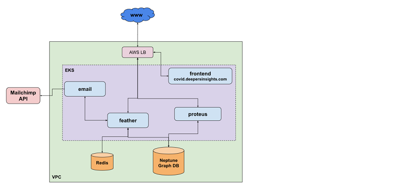
Amazon Neptune and Apache TinkerPop Gremlin
Although we initially considered setting up our own Apache TinkerPop service, none of us were experts with graph database infrastructure, and we found the learning curve around self-hosted graphs (such as JanusGraph) extremely steep given the time constraints on our project. This was exacerbated by the fact that we didn’t know how many users might be querying our graph at once, so rapid and simple scalability was another requirement. Fortunately, Neptune is a managed graph database service that allows storing and querying large graphs in a performant and scalable way. This also pushed us towards Neptune’s native query language, Gremlin, which was also a plus because it’s the language the team had most experience with, and provides a DSL for writing queries in Python, our house language.
Neptune allowed us to solve the first challenge: representing a large textual dataset as a knowledge graph that scales well to serving concurrent, computationally intensive queries. With these basics in place, we needed to build out the AWS infrastructure around the rest of the project.
Proteus
Beyond Neptune, our solution involved two API services—Feather and Proteus—to allow communication between Neptune and its API, and to the outside world.
More specifically, Proteus is responsible for managing the administration activities of the Neptune cluster, such as:
- Retrieving the status of the cluster
- Retrieving a summary of the queries currently running
- Bulk data loading
The last activity, bulk data loading, proved especially important because we were dealing with a very large volume of data, and one that will grow with time.
Bulk data loading
This process involved two steps.
The first was developing code to integrate the Python-based parsing we described earlier with a final pipeline step to convert the relevant spaCy objects—the nested data structures containing documents, entities, and spans representing predicates, subjects, and objects—into a language Neptune understands. Thankfully, the spaCy API is convenient and well-documented, so flattening out those structures into a Gremlin insert query is fairly straightforward.
Even so, importing such a large dataset via Gremlin-language INSERT statements, or addVertex and addEdge steps, would have been unworkably slow.
To load more efficiently, Neptune supports bulk loading from the Amazon Simple Storage Service (S3). This meant an additional modification to our pipeline to write output in the Neptune CSV bulk load format, consisting of two large files: one for vertices and one for edges. After a little wrangling with datatypes, we had a seamless parse-and-load process. The following diagram illustrates our architecture.
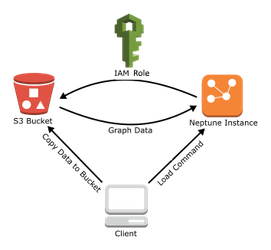
It’s also worth mentioning that in addition to the CSV format for Gremlin, the Neptune bulk loader supports popular formats such as RDF4XML for RDF (Resource Description Framework).
Feather
The other service that communicates with Neptune, Feather, manages the interaction between the user (through the front end) and Neptune instance. It’s responsible for querying the database and delivering the results to the front end.
The front-end service is responsible for the visual representation of the data provided by the Neptune database. The following screenshot shows our front end displaying our biomedical corpus.

On the left we can see the topic-based graph browser showing the concepts most closely related to COVID-19. In the right-hand panel we have the document list, showing where those relations were found in biomedical papers at the phrase and sentence level.
Lastly, the mail service allows you to subscribe to receive alerts around new themes as more data is added to the corpus, such as the COVID-19 Insights Newsletter.
Infrastructure
Owing to the Neptune security configuration, any incoming connections are only possible from within the same Amazon Virtual Private Cloud (Amazon VPC). Because of this, our VPC contains the following resources:
- Neptune cluster – We used two instances: a primary instance (also known as the writer, which allows both read and write) and a replica (the reader, which only allows read operations)
- Amazon EKS – A managed Amazon Elastic Kubernetes Service (Amazon EKS) cluster with three nodes used to host all our services
- Amazon ElastiCache for Redis – A managed Amazon ElastiCache for Redis instance that we use to cache the results of commonly run queries
Lessons and potential improvements
Manual provisioning (using the AWS Management Console) of the Neptune cluster is quite simple because at the server level, we only need to deal with a few primary concepts: cluster, primary instance and replicas, cluster and instance parameters, and snapshots.
One of the features that we found most useful was the bulk loader, mainly due to our large volume of data. We soon discovered that updating a huge graph was really painful. To mitigate this, each time a new import was required, we created a new Neptune cluster, bulk loaded the data, and redirected our services to the new instance. Additional functionality we found extremely useful, but have not highlighted specifically, is the AWS Identity and Access Management (IAM) database authentication, encryption, backups, and the associated HTTPS REST endpoints. Despite being very powerful, with a bit of a steep learning curve initially, they were simple enough to use in practice and overall greatly simplified this part of the workflow.
Conclusion
In this post, we explained how we used the graph database service Amazon Neptune with complementing Amazon technologies to build a robust, scalable graph database infrastructure to extract knowledge from a large textual dataset using high-level semantic queries.
We chose this approach since the data needed to be queried by the client at a broad, conceptual level, and therefore was the perfect candidate for a Knowledge Graph. Given Neptune is a managed graph database with the ability to query a graph with milliseconds latency it meant that the ease of setup if would afford us in our time-poor scenario made it the ideal choice.
It was a bonus that we’d not considered at the project outset to be able to use other AWS services such as the bulk loader that also saved us a lot of time. Altogether we were able to get the Covid Insights Platform live within 8 weeks with a team of just three; Data Scientist, DevOps and Full Stack Engineer.
We’ve had great success with the platform, with researchers from the UK’s NHS using it daily. Dr Matt Morgan, Critical Care Research Lead for Wales said “The Covid Insights platform has the potential to change the way that research is discovered, assessed and accessed for the benefits of science and medicine.”
To see Neptune in action and to view our Covid Insights Platform, visit https://covid.deeperinsights.com
We’d love your feedback or questions. Email info@deeperinsights.com