AWS Database Blog
Collecting, storing, and analyzing your DevOps workloads with open-source Telegraf, Amazon Timestream, and Grafana
Telegraf is an open-source, plugin-driven server agent for collecting and reporting metrics. Telegraf offers over 230 plugins to process a variety of metrics from datastores to message queues, including InfluxDB, Graphite, OpenTSDB, Datadog, and others. Customers asked us to integrate Telegraf with Amazon Timestream, a fast, scalable, serverless time series database service for IoT and operational applications, so we did. Thanks to the Timestream output plugin for Telegraf, you can now ingest metrics from Telegraf agent directly to Timestream.
In this post, you will learn how to:
- Install, configure, and run a Telegraf agent with the Timestream output plugin
- Collect your host DevOps metrics using Telegraf and write them to Timestream
- Ingest time series data in InfluxDB line protocol format through Telegraf to Timestream, without changing your application code
- Use Grafana to visualize the metrics stored in Timestream
Architecture overview
Before diving deep into our use case, let’s consider a high-level deployment architecture for using a Telegraf agent with the Timestream output plugin. The metrics flow from the source (step 1 in the following diagram), through processing (step 2), to storage, and then they are accessed (step 3).

With Telegraf, you can monitor a number of different sources: system stats, networking metrics, application metrics, message queues, and more. You can do that thanks to input plugins. For the full plugin list, see the GitHub repo. The input plugins are responsible for providing metrics from different sources to Telegraf, and can either listen or fetch metrics.
You can aggregate and process collected metrics in Telegraf and send them to the Timestream output plugin. The plugin converts the metrics from the Telegraf model to a Timestream model and writes them to Timestream. The agent can be running on-premises or in the AWS Cloud, such as on Amazon Elastic Compute Cloud (Amazon EC2) instances, in Amazon Elastic Container Service (Amazon ECS), AWS Fargate, and more.
You can query Timestream directly or by using a tool like Grafana. You can run Grafana yourself (on-premises or in the AWS Cloud), or use Grafana cloud. You configure Grafana to query Timestream through the Timestream datasource.
The detailed architecture depends on your use case. In this post, we provide an example deployment fully in the AWS Cloud.
Prerequisites
Before you begin, you must have the following prerequisites:
- An AWS account that provides access to Amazon EC2 and Timestream.
- An AWS Identity and Access Management (IAM) user with an access key and a secret access key. You must be able to configure the AWS Command Line Interface (AWS CLI) and have permissions to create:
- IAM roles and policies
- Timestream databases and tables
- EC2 instances
- Auto Scaling groups
- Stacks in AWS CloudFormation
- An Amazon Virtual Private Cloud (Amazon VPC) with a public subnet.
Solution overview
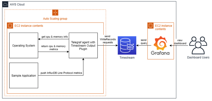
For this post, you simulate your fleet of servers by launching five EC2 instances in an Auto Scaling group.
Each EC2 instance runs a Telegraf agent and a sample application. The sample application estimates pi number using the Monte Carlo method. It sends it as an application metric in InfluxDB line protocol format to the local Telegraf agent on Amazon EC2.
The Telegraf agent, which runs on each Amazon EC2, performs three main roles:
- Uses its plugins to collect CPU and memory metrics
- Accepts writes in InfluxDB line protocol format from your application
- Writes the metrics to the Timestream database
Finally, you run Grafana and expose an operational dashboard by launching one more EC2 instance. Grafana queries Timestream and returns the result to the user in a dashboard form.
The following diagram illustrates the solution architecture for this use case.
Deploying the solution
We provide an AWS CloudFormation template in this post as an example, which you can review and customize as needed. Some resources deployed by this stack incur costs when they remain in use.
For this post, the resources are installed in a VPC with a public subnet. We recommend installing the resources in a private subnet whenever possible for production. In addition, we recommend enabling TLS connections and password authentication from your applications to Telegraf and for Grafana. To troubleshoot, the CloudFormation template sets up network inbound access to port 22 from a limited IP CIDR scope, enabling you to access EC2 instances remotely. If this is not needed, you can remove the access.
To start provisioning your resources, choose Launch Stack:
![]()
For Amazon Timestream current region availability, see the pricing page.
The CloudFormation template does the following:
- Creates a Timestream database and three tables.
- Creates an EC2 Auto Scaling group in subnets of your choice, with EC2 instance types of your choice. On each EC2 instance in the Auto Scaling group, the template:
- Installs and configures Telegraf agent.
- Downloads and configures a Python sample application as a service, which pushes the metrics in InfluxDB protocol to a local Telegraf agent.
- Creates a single EC2 instance with Grafana installed and configured as a service that connects to the pre-installed Timestream datasource. Additionally, one sample dashboard is pre-installed to visualize various metrics about the setup.
- Creates two Amazon EC2 security groups: one for EC2 instances in the Auto Scaling group, and one for the Grafana EC2 instance. You can configure network access to inbound TCP ports 22 (SSH), Grafana (3000) with parameters in the CloudFormation template. This locks down access to the launched EC2 instances to known CIDR scopes and ports.
- Creates two IAM instance profiles: one associated with the Auto Scaling group instances (with write permissions to Timestream), and one associated with the Grafana instance (with Timestream read permissions).
Installing the Telegraf agent with the Timestream output plugin
We wrote the Timestream output plugin and contributed to the Telegraf repository. The pull request was merged and as of version 1.16, the Timestream output plugin is available in the official Telegraf release. To install Telegraf on your system, see Telegraf Installation Documentation. You can also use the following script to install Telegraf on an Amazon Linux 2 EC2 instance:
Configuring the Telegraf agent
We want Telegraf to retrieve the memory and CPU metrics, accept InfluxDB write requests, and write the data to Timestream. The following command generates an example configuration:
The generated sample.conf file contains example configuration that you can adjust to your preferences. However, you must adjust the following keys:
- Under the
[[outputs.timestream]]section, set thedatabase_nameto the name of the created Timestream database. - Under the
[[inputs.influxdb_listener]]section, comment out with the # character the following keys:tls_allowed_cacerts,tls_cert, andtls_key. This is to simplify the example. We advise that you use TLS certificates in your production environment.
The configuration also defines how the metrics are translated from Telegraf (InfluxDB) to the Timestream model. The plugin offers you two modes, which you can use by changing the mapping_mode key. For more information, see Configuration.
Running the Telegraf agent
When you have the configuration file, you can run Telegraf with the following command:
However, if you run Telegraf as a service, it automatically restarts if there are issues. You can run the Telegraf as a service and check the service status with the following commands on Amazon Linux 2 EC2 instance:
Using InfluxDB line protocol to write to Timestream through Telegraf
For this post, we wrote a Python application that constantly estimates pi number and sends the metric to the InfluxDB database. See the following code:
The sample application connects to the InfluxDB server and sends the pi estimation and iteration number to the InfluxDB every second. Native InfluxDB libraries are used to submit the metrics. With a Telegraf InfluxDB listener, you can use the same code that you’re using now to ingest data to Timestream. All you have to do is change the host and port in your configuration to your Telegraf agent.You can run the sample application with the following code:
You can refer to the setup_sample_application.sh script to download and configure the Python sample application as a Linux service on Amazon Linux 2.
The ingestion setup is now complete.
Setting up Grafana with a Timestream datasource
We have prepared the setup-grafana.sh script to download, install, and configure Grafana with a Timestream datasource and a sample dashboard.
You can also set up Grafana with a Timestream datasource manually. For instructions, see Using Timestream with Grafana.
Browsing the metrics in Timestream
A few minutes after you launch the CloudFormation stack, you should see a new database in Timestream. On the AWS CloudFormation console, choose your stack, and choose the Outputs tab. There, you can see the TimestreamDatabaseName key with the new database name in the value column.
On the Timestream console, navigate to the databases view and choose your database. You can see the following tables in your Timestream database:
cpu(withhostandcpudimensions,measure_value::double,measure_name, andtime)mem(withhostdimension,measure_value::bigint,measure_value::double,measure_name, andtime)sample_app(withhostandsession_uuiddimensions,measure_value::bigint,measure_value::double,measure_name, andtime)

You can choose the three dots near the table name, and choose Show measures to explore what measures are stored in a table. For example, the following screenshot shows the measures from the sample_app table: iteration (data_type bigint, with host and session_uuid dimensions), and pi (data_type double, with host and session_uuid dimensions).

Browsing the metrics in Grafana
After launching the CloudFormation stack, on the AWS CloudFormation console, choose your stack and choose the Outputs tab to see the GrafanaURL key. Navigate to the URL in the value column. You had to specify your public IP address when launching the stack to be able to access the Grafana URL. Also, keep in mind that your VPN or proxy can block the access to 3000 port.
Log in to Grafana using the default admin/admin credentials and open My π Estimation DevOps Dashboard. You should see a view showing you several panels:
- last average π estimate – Value is 3.14588
- π estimate per host graph – Values converging to π value
- π iteration count per host – Values around 1500
- cpu-total: usage_system per host graph – Minimal CPU usage
- cpu-total: usage_user per host graph – Minimal CPU usage
- memory: available_percent per host – Values depend on your EC2 instance type
- memory: free per host – Values depend on your EC2 instance type

Choose the panel title and choose Edit to explore the Timestream query for a particular panel. For example, the π estimate per host panel query looks like following code:
Cleaning up
To avoid incurring future charges, delete the CloudFormation stack that you created.
Conclusion
In this post, you learned how to use Telegraf to send DevOps metrics to Timestream. You also learned how to use Telegraf as a proxy to translate InfluxDB writes to Timestream without modifying your applications.
Check out the Timestream output plugin for Telegraf and try ingesting data from your real applications to Timestream.
About the author

Piotr Westfalewicz is a NoSQL data architect at AWS. He is passionate about building the right solution for customers. Before working as a data architect, he was a software development engineer at both Amazon and AWS.