Novartis AG uses Amazon SageMaker and Amazon Neptune to build and enrich a knowledge graph using BERT (Part 2/4)

September 8, 2021: Amazon Elasticsearch Service has been renamed to Amazon OpenSearch Service. See details.

This is the second post of a four-part series on the strategic collaboration between AWS and Novartis AG, where the AWS Professional Services team built the Buying Engine platform.

In this series:

Part 1: How Novartis AG brought SMART into Smart Procurement with AWS Machine Learning
Part 2: Novartis AG uses Amazon SageMaker and Amazon Neptune to build and enrich a knowledge graph using BERT (this post)
Part 3: Novartis AG uses Amazon OpenSearch Service K-Nearest Neighbor (KNN) and Amazon SageMaker to power search and recommendation
Part 4: Demand Forecasting with Amazon SageMaker and GluonTS at Novartis AG

This post focuses on the Knowledge Base of the Buying Engine, which provides business analysts with a complete view on catalog data, along with insights. We go into detail about how Novartis AG uses Amazon SageMaker with TensorFlow 2 and Amazon Neptune to build and enrich an in-house knowledge base.

Amazon SageMaker is a fully managed service that provides developers and data scientists with the ability to build, train, and deploy machine learning (ML) models quickly. Amazon SageMaker removes the heavy lifting from each step of the machine learning process to make it easier to develop high-quality models. The SageMaker Python SDK provides open source APIs and containers that make it easy to train and deploy models in Amazon SageMaker with several different machine learning and deep learning frameworks. We use an Amazon SageMaker Notebook Instance for running the code. For information on how to use Amazon SageMaker Notebook Instances, see the AWS documentation.

Amazon Neptune is a fast, reliable, fully managed graph database service that makes it easy to build and run applications that work with highly connected datasets. The core of Neptune is a purpose-built, high-performance graph database engine. This engine is optimized for storing billions of relationships and querying the graph with milliseconds latency. Neptune powers graph use cases such as recommendation engines, fraud detection, knowledge graphs, drug discovery, and network security.

Project motivation

To build the knowledge base, we considered several options – Amazon Neptune, Amazon DynamoDB or Amazon S3. Working backwards from the customer requirements, we found the use case can be better addressed using a knowledge graph on Amazon Neptune. A knowledge graph captures the semantics of a particular domain using a set of definitions of concepts, their properties, relations between them, and logical constraints that are expected to hold. For instance, relevancy and connection between products and properties can be better identified when viewed as a graph. This can lead to better item selection and recommendation. Additionally, a graph can contain multiple layers that get enriched in the process (i.e. product layers, click-stream data layer). For more information see Knowledge Graphs on AWS.

The Buying Engine catalogue contains products from a variety of vendors and suppliers. Ensuring consistency is a challenge when building such a centralized graph representation, as products are often composed of unstructured text descriptions and inconsistent property mappings. To address this challenge, we leverage SageMaker to build and train a custom Named Entity Recognition (NER) model based on BERT. This lets us extract product attributes and use them as standardized inputs for the knowledge graph.

In this post, we provide technical guidelines on building and enriching a knowledge graph using NER techniques for data scientists working on similar challenges.

The reminder of this post guides you through the following steps: (1) notebook setup (2) custom train script for NER BERT on SageMaker (3) custom inference script to deploy inference at scale on SageMaker (4) knowledge graph setup and querying with Neptune.

Setting up

Create an S3 bucket. This will be used throughout the notebooks to store files generated by the examples.
Create a SageMaker notebook instance. Please observe the following:
- The execution role must be given an additional permission to read/write from the S3 bucket created in step 1.
- If you put the notebook instance inside a Virtual Private Cloud (VPC), make sure that the VPC allows access to the public Pypi repository and aws-samples/ repositories.
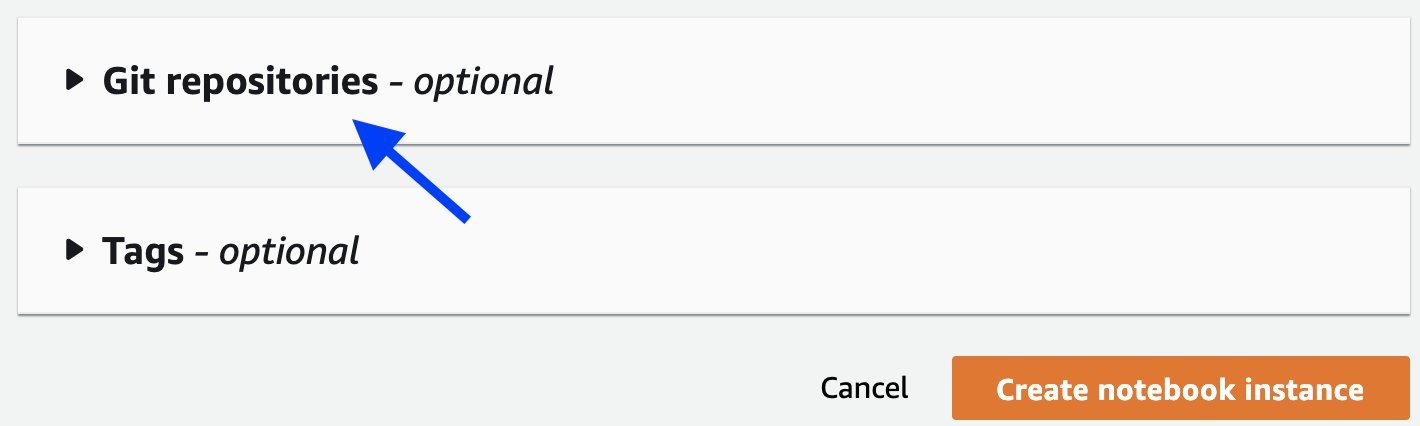
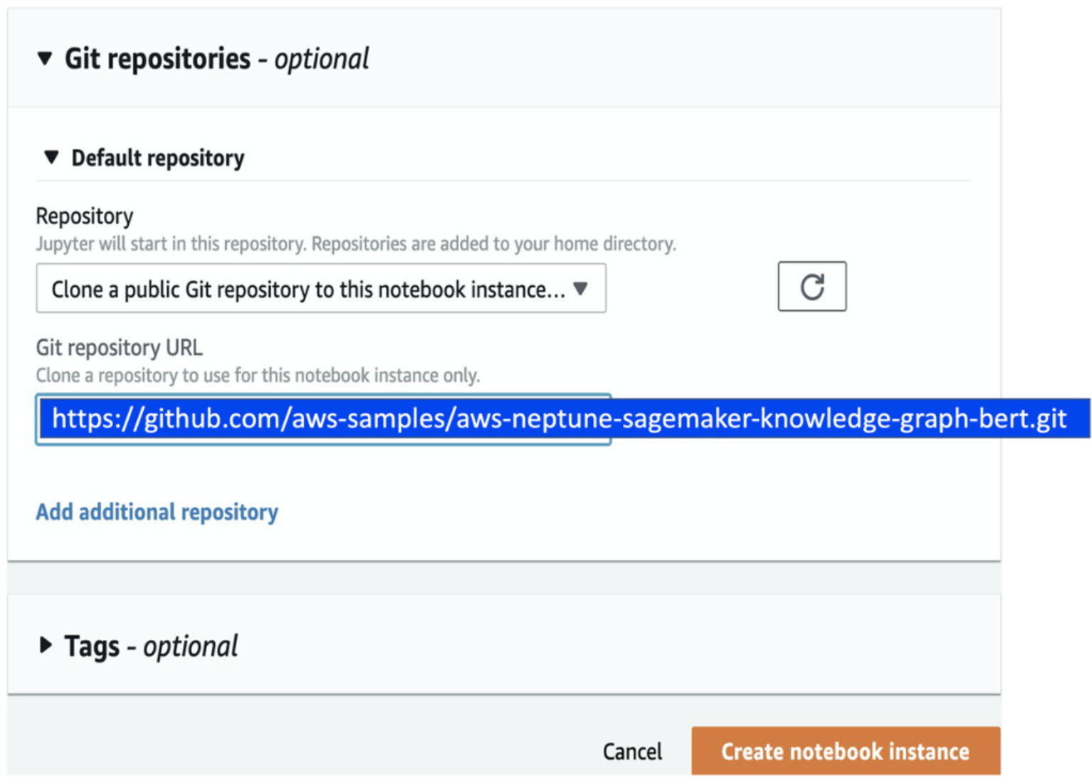
- Attach this Git repository to the notebook, as shown in the following screenshots.

Training a NER model using BERT and Amazon SageMaker

For building the Named Entity Recognition algorithm, we decided to use BERT, a widely known NLP model leveraging transfer learning with a base architecture of Transformer encoders pre-trained on a large corpus of text. This lets us tune it to our specific task and data, like Named Entity Recognition for lab supplies product characteristics.

We were inspired by pos-tagger-bert on GitHub, an excellent and comprehensive introduction to using BERT for Named Entity Recognition with Keras and TensorFlow 2.

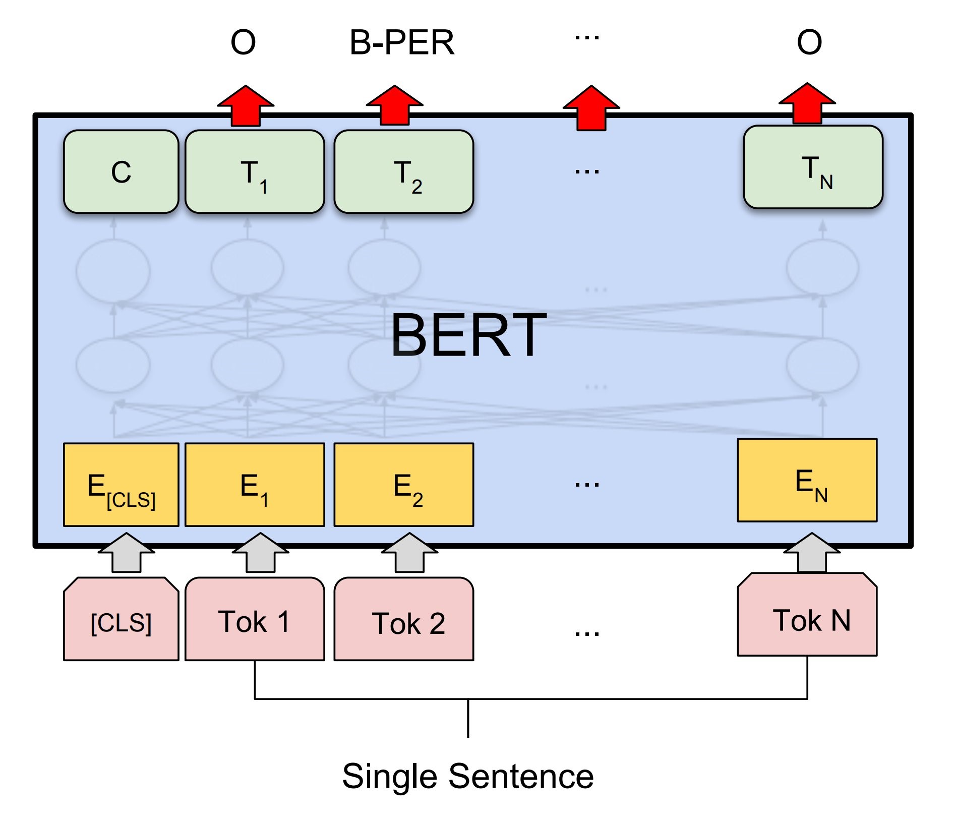
Illustration taken from arXiv:1810.04805

Given the level of customization and flexibility that was required, we decided to leverage Amazon SageMaker Python SDK for building custom deep learning models. This let us use a pre-built Amazon SageMaker TensorFlow container. Then, we could simply integrate the training and inference code.

To do this, you start by specifying a training entry point that will apply the necessary preprocessing for BERT. Then, build and train the model using Keras. Finally, save the weights and architecture into the adequate format to be used by the SageMaker TensorFlow Serving container.

To make the code more readable, most functions are saved into modules in the folder “source” of the repository.

Creating a train script to run with SageMaker script mode

Preprocessing for BERT

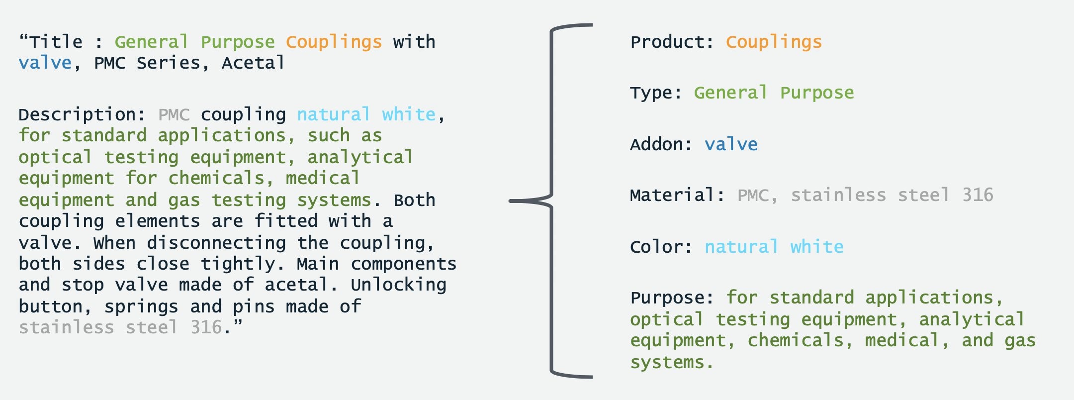
BERT expects inputs to be in the form of lists of words. For example, the product description “General Purpose Couplings with valve, PMC Series, Acetal” along with tags associated to it, is transformed into the following list:

[(“General”, Type), (“Purpose”, Type), (“Couplings”, Product), (“with”, Other), (“valve”, Addon), (“PMC”, Other), (“Series”, Other), (“Acetal”, Other)],

BERT’s input is constrained by a maximum sequence length. Sometimes this results in splitting long descriptions into the appropriate length. For illustration purposes, the max_sequence_length of 3 would produce:

[[(“General”, Type), (“Purpose”, Type), (“Couplings”, Product)],

[(“with”, O), (“valve”, Addon), (“PMC”, O)],

[(“Series”, O), (“Acetal”, O)],

By default, BERT’s max input length is 512. However, the computation time increases quadratically with respect to the length of the input. Because of this, there is a sweet spot to find when using a large input to take advantage of a larger context (increasing accuracy). Using a shorter input makes both training and inference more efficient (increasing speed). In practice, we found that a max_sequence_length of 64 gives good results while keeping computation needs relatively low.

Finally, to feed into BERT, words are tokenized using a WordPiece tokenizer. This tokenizer may cut words into two or more subwords (Johnson → John ##son) if it encounters a word out of the vocabulary used in its training. Using the tokenizer, each word in a description is transformed into input_ids (the vocabulary id of the word/subword). Alongside those, BERT requires input_mask (distinguishing between padding inputs and real words) and segment_ids (here simply set to 0). The code also generates label_ids by transforming the labels into one-hot encoded vectors, which will be the target of the training task.

# Read the data
train_sentences = pd.read_csv(os.path.join(args.train, 'train.csv'), engine='python')
val_sentences = pd.read_csv(os.path.join(args.validation, 'val.csv'), engine='python')

# Create the labels dictionnaries from the data
tag2int, int2tag = prepro.create_tag_dictionnaries(train_sentences, val_sentences)

# Reading the parameters passed to the training job and saving for inference
MAX_SEQUENCE_LENGTH=args.max_sequence_length
BERT_PATH=args.bert_path

save_parameters_for_inference(MAX_SEQUENCE_LENGTH, BERT_PATH, tag2int, int2tag)

# Sequence pre-processing
# Splitting the sequences
train_sentences, val_sentences = prepro.split(train_sentences, val_sentences, MAX_SEQUENCE_LENGTH)

# Separating text and labels
train_text, val_text  = prepro.text_sequence(train_sentences, val_sentences)
train_label, val_label = prepro.tag_sequence(train_sentences, val_sentences)

# BERT pre-processing
# Instantiate tokenizer
tokenizer = prepro.create_tokenizer_from_hub_module(BERT_PATH)

# Convert to BERT features
(train_input_ids, train_input_masks, train_segment_ids, train_labels
) = prepro.convert_examples_to_features(tokenizer,
                                        train_text,
                                        train_label,
                                        tag2int,
                                        max_seq_length=MAX_SEQUENCE_LENGTH+2)
(val_input_ids, val_input_masks, val_segment_ids, val_labels
) = prepro.convert_examples_to_features(tokenizer,
                                        val_text,
                                        val_label,
                                        tag2int,
                                        max_seq_length=MAX_SEQUENCE_LENGTH+2)

To make sure that the preprocessing is the same during inference and training, save the pre-processing parameters at this step. This saves under the SM_MODEL_DIR folder, alongside the training weights that are later generated. These are saved in Amazon S3 bucket you specify at the end of the training job. Everything needed to deploy the trained model as a SageMaker model afterwards is saved in SM_MODEL_DIR.

Model building and training

Once the conversion to BERT inputs is over, the model is built and trained using Keras.

To load the BERT pre-trained weights from TensorFlow hub, here the default uncased English BERT is used. The detail of the architecture can be found in the source code.

#Building a keras model based on the previous section
model = build_model(max_seq_length = MAX_SEQUENCE_LENGTH+2,
                            n_tags=len(tag2int),
                            lr=args.learning_rate,
                            drop_out=args.drop_out,
                            bert_path=args.bert_path,
                            loss=args.loss
                            )
model_dir = "/opt/ml/model"
checkpoint = ModelCheckpoint(filepath=os.path.join(model_dir, "ner_model.h5"),
                        monitor='val_acc',
                        save_best_only=True,
                        save_weights_only=True,
                        verbose=1)

history = model.fit(training_data=([train_input_ids, train_input_masks, train_segment_ids], train_labels),
                    validation_data=([val_input_ids, val_input_masks, val_segment_ids], val_labels),
                    epochs=args.epochs,
                    batch_size=args.batch_size,
                    shuffle=True,
                    verbose=1,
                    callbacks=[checkpoint,
                               EarlyStopping(monitor = 'val_accuracy', patience = 5)])

Saving the model for TensorFlow Serving

Once the training is over, the best weights are loaded. The model alongside the weights is converted to the Protobuff format and saved into the right folder to be used by the SageMaker TensorFlow Serving container. The code below details how to save the model:

# Reload best saved checkpoint: 
model.load_weights(os.path.join(model_dir, 'ner_model.h5')) 

# Note: This directory structure will need to be followed
model_version = '1'
export_dir = os.path.join(model_dir, 'model/', model_version)

tf.saved_model.save(obj=model, export_dir=export_dir)

Creating an Inference script to extract product properties

Once the NER model has been trained, move onto generating product properties to create the knowledge graph.

To run inference at scale either by deploying a SageMaker Endpoint or run Batch Inference, we need to create an inference script that works with the Tensorflow SageMaker container that gets created through the SageMaker Python SDK. In the following section we show how to build this script.

PyTorch and Apache/MXNet SageMaker containers let you specify how to load a model by modifying the model_fn. On the other hand, the model deployment for SageMaker TensorFlow Serving containers is “implicit” and expects the folder structure and naming that has been defined in the previous section. However two functions can be modified to deal with specific input and output processing namely input_handler and output_handler. This is where you place the specific BERT input preprocessing and perform some output formatting.

Loading preprocessing parameters

The first step of our inference script is reading the parameters dumped during training to reproduce the preprocessing and instantiate the same tokenizer. To avoid a tokenizer instantiation each time you call the model, it is crucial to place it outside the input_handler and output_handler functions.

# Reading BERT processing input parameters
with open('/opt/ml/model/int2tag.json') as f:
    int2tag = json.load(f)
with open('/opt/ml/model/tag2int.json') as f:
    tag2int = json.load(f)

n_tags = len(tag2int)

with open('/opt/ml/model/max_sequence_length.txt') as f:
    MAX_SEQUENCE_LENGTH = int(f.read())

with open('/opt/ml/model/bert_path.txt') as f:
    bert_path = f.read()

# Instantiate tokenizer (outside input_handler())
tokenizer = create_tokenizer_from_hub_module(BERT_PATH)

Input handler

The input handler function is called upon each prediction request. The textual data specified in the prediction payload goes through the same preprocessing used in the training phase. This generates the “inputs” tensor, which is then sent to the TensorFlow Serving REST API. The following code details the data processing before it reaches the model:

def input_handler(data, context):
    if context.request_content_type == 'application/json':
        d = json.load(data)

    # Splitting input into words
    global sentences
    sentences = [line.split() for line in d]

    # Sentence preprocessing (split with max sequence length)"
    global split_sentences
    global split_idx
    split_sentences, split_idx = prepro.split_and_duplicate_index(sentences,
                                                                  MAX_SEQUENCE_LENGTH)

    # Creating tags placement for unlabelled data (-PAD-)")
    tags_placement = []
    for sentence in split_sentences:
        tags_placement.append(['-PAD-']*len(sentence))

    # BERT pre-processing
    (input_ids, input_masks, segment_ids, _
    ) = prepro.convert_examples_to_features(tokenizer,
                                            split_sentences,
                                            tags_placement,
                                            tag2int,
                                            max_seq_length=MAX_SEQUENCE_LENGTH+2)

    # Convert BERT features to necessary format for TensorFlow Serving
    input_ids = input_ids.tolist()
    input_masks = input_masks.tolist()
    segment_ids = segment_ids.tolist()

    result={
    'inputs':{
        "input_word_ids": input_ids,
        "input_mask": input_masks,
        "input_type_ids": segment_ids
        }
    }

    return json.dumps(result)

With BERT requiring to split descriptions when larger than the input size of the model, it is important to be able to keep track of the original descriptions. In order to achieve this, split_and_duplicate_index() creates an index for each of the original sequence that will be later used for mapping back the predictions to their original description. Both the index and original sequence are saved as global variables to be available for the output_handler.

Output Handler

After the inputs generated by the input_handler are sent to the model, the TensorFlow model outputs predictions in the form of arrays of numbers corresponding to the tag indexes. The output_handler allows us to add a few post-processing steps (i.e. converting predictions back to their label, regroup split sentences, and transform each sequence prediction into a readable dictionary of tag and values).

def output_handler(data, context):
    if data.status_code != 200:
        raise ValueError(data.content.decode('utf-8'))

    # Reading model predictions as data.content
    response_content_type = context.accept_header
    prediction = data.content
    pred = json.loads(prediction.decode('utf-8'))
    
    # Select the tag prediction with the highest score for each word
    pred_max = [list(np.array(k).argmax(-1)) for k in pred['outputs']]
    
    # Convert label_ids (y) to labels
    y_pred = postpro.y2label(pred_max, int2tag, mask=0)
    
    # Remapping split sequences to origin index"
    flat_y_pred, _ = postpro.map_split_preds_to_idx(y_pred, split_idx)
    
    # Format output to dicts for compatibility with Knowledge graph
    nerc_prop_list = [postpro.preds_to_dict_single_lower(s,y) for s,y in zip(sentences,flat_y_pred)]
    pred_dict_list = [{'ner_properties':nerc_prop_list[i]} for i, x in enumerate(sentences)]

    return json.dumps(pred_dict_list), response_content_type

When the inference script is built this way, populating the knowledge graph is simplified. Each product is associated with a number of characters with values attached. (This is illustrated in the first image in this blog post.)

Building and enriching the knowledge graph

Amazon Neptune is a fast, reliable, fully managed graph database service that makes it easy to build and run applications that work with highly connected datasets. Amazon Neptune is purpose-built for storing billions of relationships and querying the graph with milliseconds latency. In our use case we model the data using Resource Description Framework and query using SPARQL.

After extracting product properties from product descriptions, you can define the knowledge graph model, set up Amazon Neptune, and perform queries using SPARQL. For the complete code for data handling, see the GitHub repository.

Knowledge graph model

A formally structured graph model can represent a product and values it has. This includes: properties represented by hasProperty relationship; and other fields of the product like price, manufacturer, and currency.

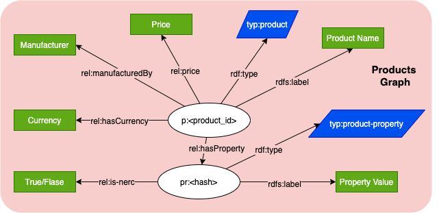
Each property is represented by a node, type (i.e. color, material), and value. It also includes a flag if this property was a result from NER model or if it is a defined property from the vendor data. A combination of property value and property type is used as a unique identifier for the property node. With this, it can be referenced by other products.

Setting up Amazon Neptune

To set up a Neptune cluster, you can use a CloudFormation stack and refer to the Getting started with Neptune documentation. Once the stack has been deployed, you can check the status of your Neptune instance.

The NER model output is then fed to Neptune as the graphical database to build the knowledge graph. SPARQL was the language of choice in our project, so the JSON output was translated to RDF triplets.

Once the triplets are created as defined in the graph model, use Neptune’s load endpoint to perform a bulk load.

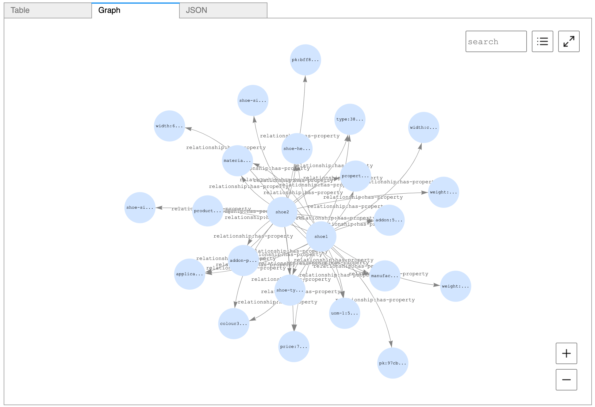
Querying Neptune using SPARQL

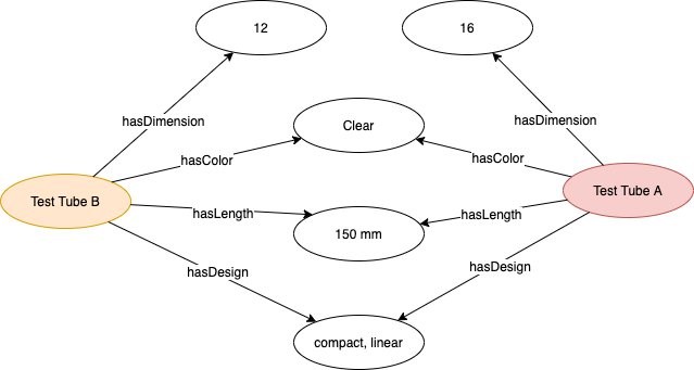
Use the Neptune workbench to run queries over the graph. For example, to find similar products based on how many connections in common a product with id-012345 has with other products, the following query can be used:

BASE <http://example.com/>

PREFIX pr: <resource/product/>

SELECT ?similar (COUNT(?p) as ?similarity) ( group_concat(?p; separator=",") as ?relationships) 
FROM <products>
WHERE {
    VALUES ?product { pr:012345 }
    ?similar ?p ?o .
    ?product ?p ?o .
}
GROUP BY ?similar ?product
HAVING ( COUNT(?p) > 1 )
ORDER BY DESC(?similarity)
LIMIT 5

The following image shows the output of this query:

The following image shows how the top two products are visualized from Neptune workbench:

Cleaning up

When you finish this exercise, remove your resources with the following steps:

Delete your notebook instance and the endpoint created
Optionally, delete registered models
Optionally, delete the SageMaker execution role
Optionally, empty and delete the S3 bucket, or keep whatever you want

Summary

You should now have the foundational knowledge to build a custom Named Entity Recognition model using BERT with SageMaker script mode to run training and inference at scale. Additionally, these predictions can be used to build a knowledge graph that you can query to analyze and extract insights about the products on Neptune.

The AWS Professional Services model provided the opportunity to deliver a production-ready ML solution from which you have seen an extract in this blogpost. It also gave us the chance to train the Novartis AG team on productionizing ML best practices so that they can maintain, iterate, and improve upon their ML efforts. With the resources provided, they can expand to other possible future use cases.

Get started today! You can learn more about SageMaker and kick off your own machine learning solution by visiting the Amazon SageMaker console.

AWS welcomes your feedback. Feel free to leave us any questions or [1] comments.

Many thanks to the Novartis team who worked on the Buying Engine project. Special thanks to following, who contributed to this blog post:

Srayanta Mukherjee: Srayanta is the Director of Data Science on the Data Science & Artificial Intelligence team at Novartis. He was the data science lead during the delivery for the Novartis Buying Engine.
Petr Hantych: Petr is a Principal Data Scientist at Novartis IT, working on projects from the very beginning up until delivering final application. In spare time he is enjoying any triathlon race he does not finish last.
Adithya N: Adithya is a Data Scientist at Novartis IT who works on developing Data Science solutions, right from the inception stage to industrialization stage. In his free time, Adithya enjoys playing multiple musical instruments, playing chess and reading books in the genre of behavioral economics.