Artificial Intelligence
Benchmarking Training Time for CNN-based Detectors with Apache MXNet
This is a guest post by Cambron Carter, Director of Engineering, and Iris Fu, Computer Vision Scientist at GumGum. In their own words, “GumGum is an artificial intelligence company with deep expertise in computer vision, which helps their customers unlock the value of images and videos produced daily across the web, social media, and broadcast television.”
The state-of-the-art in object detection
Detection is one of many classic computer vision problems that has significantly improved with the adoption of convolutional neural networks (CNNs). When CNNs rose to popularity for image classification, many relied on crude and expensive preprocessing routines for generating region-proposals. Algorithms like Selective Search were used to generate candidate regions based on their “objectness” (how likely they are to contain an object) and those regions were subsequently fed to a CNN trained for classification. While this approach produces accurate results, it has a significant runtime cost. CNN architectures like Faster R-CNN, You Only Look Once (YOLO), and Single Shot MultiBox Detector (SSD) address this tradeoff by embedding the localization task into the network itself.
In addition to predicting class and confidence, these CNNs attempt to predict the extrema of regions containing certain objects. In the case of this post, these extrema are simply the four corner points of a rectangle, often referred to as a bounding box. The previously mentioned detection architectures require training data which has been annotated with bounding boxes, i.e. this image contains a person and that person is within this rectangular region.
| Classification training data | Detection training data |
 |
 |
| Extraordinarily handsome and capable engineer | Extraordinarily handsome and capable engineer |
We sought out to compare the experience of training SSD using Apache MXNet and Caffe. The obvious motivation is to train these new architectures in a distributed fashion without suffering a reduction in accuracy. For more info on the architecture, have a look here, see “SSD: Single Shot MultiBox Detector.”
Tools for training
For this set of experiments, we tried several NVIDIA GPUs: Titan X, 1080, K80, and K520. We host a gang of Titan Xs and 1080s in house, but also use AWS GPU-based EC2 instances. This post is restricted to the g2.2x and p2.8x instance types. Luckily for us, there were already some available implementations of SSD using MXNet, such as this, which we used for the experiments in this discussion. It is worth noting that for the experiment to be exhaustive, you should include benchmarking data for other popular frameworks, such as TensorFlow.
Speed: The effect of adjusting batch size and GPU count with MXNet
First and foremost, let’s have a look at the performance impact of multi-GPU training sessions using MXNet. These first experiments are focused on training SSD with MXNet on EC2 instances. We use the PASCAL VOC 2012 dataset. The purpose of this first exercise is to understand the effects that GPU count and batch size have on speed for a particular GPU. We used several different GPUs to illustrate their absolute performance differences. If you want to explore further, there’s a lot of information about the price and performance of different GPUs. Let’s start with K520s, which ships with g2.2x instances:
| Instance Type | GPU Card | GPUs | Batch Size | Speed (samples/sec) | Total Time for 240 Epochs (Hrs) | Epoch/Hr |
| g2.2x large | K520 | 1 | 16 | 10.5 | 118 | ~2 |
| g2.2x large | K520 | 2 | 16 | 9.83 | 112 | ~3 |
| g2.2x large | K520 | 5 | 16 | 9-10 | 38 | ~6 |
Note that, given a constant batch size, adding extra g2.2x instances (each with one K520) results in a roughly constant speed per machine. As such, the number of epochs per hour increases almost linearly. Adding machines should continue to decrease our runtime, but at a point there could be a cost in accuracy. We don’t explore this here, but it is worth a mention.
Next, we wanted to check if this trend was observed on our local 1080s:
| Instance Type | GPU Card | GPUs | Batch Size | Speed (samples/sec) | Total Time for 240 Epochs (Hrs) | Epoch/Hr |
| In-house | GTX 1080 | 1 | 16 | 48.8 | 24 | ~10 |
| In-house | GTX 1080 | 2 | 16 | 8.5 | ~ 80 | ~3 |
As expected, one 1080 outperforms five K520s with ease. Apart from that observation, this experiment raised some eyebrows. We found a tremendous reduction in per-GPU speed when adding a second 1080 into the mix. Because interprocess communication in this experiment happens over the Ethernet, we first thought that we were being throttled by our office network. According to Iperf, this hypothesis doesn’t hold:
| Iperf between: | Interval | Transfer | Bandwidth |
| Local GTX 1080 and Local GTX 1080 | 0.0-10s | 1012 MB | 848 Mb/sec |
| g2.2x large K520 and g2.2x large K520 | 0.0-10s | 867 MB | 727 Mb/sec |
Our tests show that both the bandwidth and transfer are higher in our office network than between two EC2 instances. Our next question: What if batch size is the cause of the resulting inefficiency?
| GPU Card | GPUs | Batch Size | Speed (samples/sec) | Total Time for 240 Epochs (Hrs) | Epoch/Hr |
| GTX 1080 | 2 | 16 | 8.5 | ~80 | ~ 3 |
| GTX 1080 | 2 | 32 | 15.4 | 42 | ~ 5 |
Ah-ha! Although still far slower than with one 1080, an increase in batch- along with an additional 1080 (on a separate machine) results in a speed increase. Let’s check the impact of training on a single machine with multiple, interconnected GPUs:
| GPU Card | GPUs | Batch Size | Speed (samples/sec) | Total Time for 240 Epochs (Hrs) | Epoch/Hr |
| Titan X | 1 | 32 | 40.2 | ~ 34 | ~ 7 |
| Titan X | 2 | 32 (tech 16 on each GPU) | 70.8 | ~ 20 | ~ 12 |
| Titan X | 4 | 32 (tech 8 on each GPU) | 110 | ~ 12 | ~ 20 |
We used our in-house NVIDIA DevBox, which houses four Titan Xs. Holding batch size constant but increasing the number of GPUs (technically reducing the individual batch size for each GPU), increases speed roughly 2.5x! This begs the obvious question: What if we increase the batch size per GPU?
| GPU Card | GPUs | Batch Size | Speed (samples/sec) |
| Titan X | 1 | 16 | 35.57 |
| Titan X | 2 | 32 (tech 16 on each GPU) | 70.8 |
We observe that when we keep the batch size constant (at 16) and increase the number of GPUs on the same machine, the resulting speed also increases roughly 2x. We wanted to explore this a bit further, but the buzzing of our DevBox fans kept our batch sizes at bay. The curious case of our 1080 experiment remains open, immortalized as an open issue. A potential solution on AWS might be to use placement groups, which we don’t explore in this post.
Accuracy: The effect of adjusting batch size with MXNet
Because we are tinkering with batch size so much, it is worth exploring how tinkering affects accuracy. The goal is simple: We want to reduce training time as much as possible while maintaining accuracy. We conducted this set of experiments on an in-house dataset that we use for logo detection. We carried them out on a p2.8x large instance with MXNet. We consider a detection a true positive if the intersection-over-union between the detected region and ground truth is at or above 20%. First, we tried a batch size of 8:
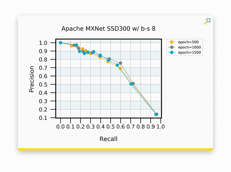
The precision and recall curve at three different stages of training. SSD uses input dimensions of 300×300 pixels, and our batch size is 8.
If we weight precision and recall equally, this leaves us at an operating point of roughly 65% for each. Let’s see what happens when we adjust the input dimensions in SSD using MXNet:
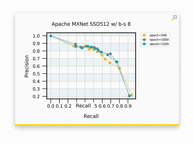
SSD using input dimensions of 512×512 pixels, with all else held constant from the previous experiment.
Here we actually see an improvement in performance, with an operating point around approximately 70% for both precision and recall. Sticking with input dimensions of 512×512 pixels, let’s investigate what adjusting batch size does to accuracy. Again, the goal is to maintain accuracy while squeezing out as much runtime as possible.
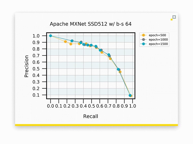
SSD using input dimensions of 512×512 pixels and a batch size of 64. Accuracy is comparable to previous experiments.
Yet again! Accuracy remains consistent, and we can reap the benefits of reduced training time with our larger batch size. In the spirit of science, let’s push it even further…

SSD using input dimensions of 512×512 pixels and a batch size of 192. Accuracy is comparable to previous experiments.
Very much the same, although our operating accuracies have fallen a bit when compared to the previous curve. Nonetheless, we have managed to generally retain accuracy while increasing batch size by 24x. To reiterate, each of these experiments was performed on a p2.8x large instance with SSD implemented on MXNet. Here’s a summary of batch size experiments, which shows comparable accuracies across experiments:
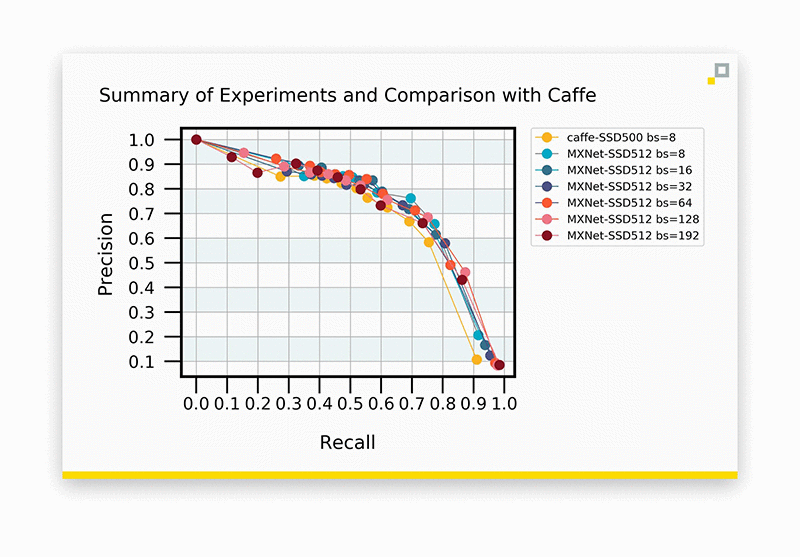
MXNet’s SSD is comparably accurate to an SSD trained with Caffe.
The takeaway is that accuracy is comparable. Getting back to the point, let’s investigate training times:
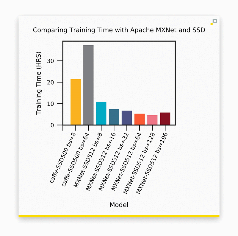
Summary of training times for Caffe and MXNet using multiple batch sizes.
The expected reduction in training time when batch size increases is obvious. However, why is there a drastic increase in training time when we increase batch size in Caffe?! Let’s have a look at nvidia-smi for both of the Caffe experiments:
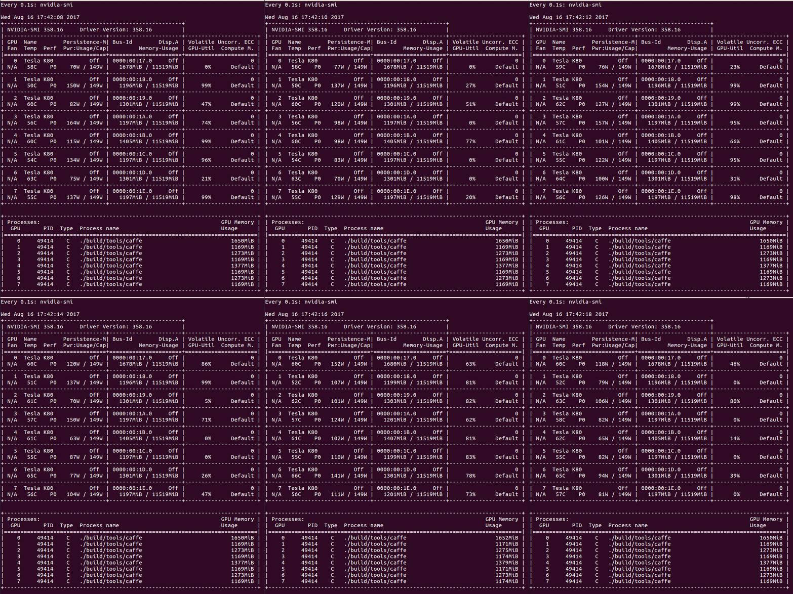
Output of nvidia-smi when training with Caffe, using a batch size of 8. Note the fluctuating GPU usage.
The GPU handles the heavy computational cost of backpropagation, which is reflected as a spike in usage. Why does usage fluctuate? It could be that the fluctuation illustrates the effect of shipping batches of training data from the CPU to the GPU. In that case, usage drops to 0% while the GPU is waiting for the next batch to be loaded. Let’s inspect the usage after doubling the batch size to 16:
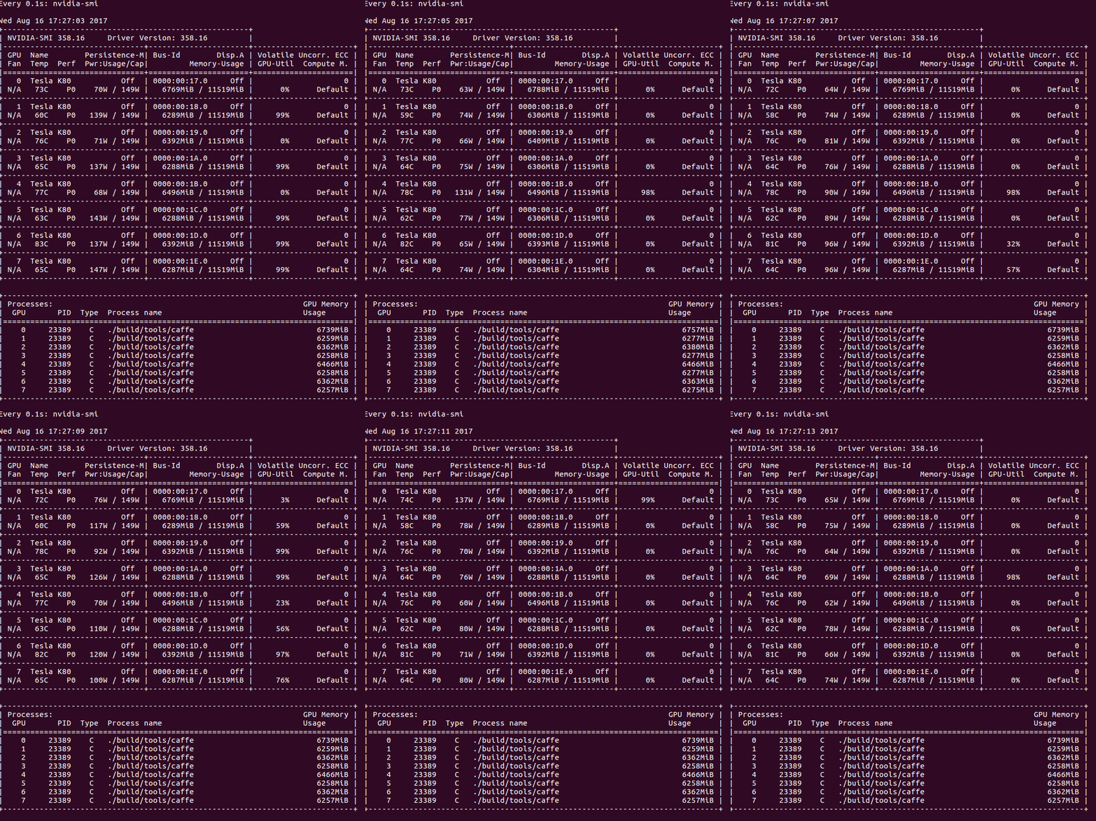
Output of nvidia-smi while training with Caffe, using a batch size of 16.
The lulls in usage are far more exaggerated and reveal an obvious inefficiency. This explains our observed increase in training time after increasing the batch size. This is nothing new or unexpected. In fact, we have also encountered this issue while training Siamese-VGG networks with Keras (and a TensorFlow backend). Discussions on this topic generally gravitate toward “the more complex your model is, the less you’ll feel the CPU-to-GPU bottleneck.” Although this is true, it isn’t very helpful. Yes, if you give the GPU more work by way of more gradients to compute, you’ll certainly see average GPU utilization increase. We don’t want to increase the complexity of our model, and, even if we did, that’s not going to help us achieve our overall goal. Our concern here is absolute runtime, not relativity.
To summarize our experiments, training time for SSD with Caffe is far higher than with the MXNet implementation. With MXNet, we observe a steady decrease in training time until we reach critical mass with a batch size of 192. We went from 21.5 hours of training time to 4.6 simply by adopting MXNet. We observed no degradation in accuracy while doing so. This is not at all a knock on Caffe—a framework that we hold near and dear—but rather a high five for MXNet. We could attack the data loading issue in a number of ways. Perhaps Caffe2 has even addressed this. Point being, we didn’t need to, and if there’s anything that will warm the heart of a machine learning developer, it’s writing the least amount of code possible. Although we still have a few unanswered questions, that’s natural when adopting a new tool. We are more than happy being guinea pigs, and are excited about the future of MXNet.
About the Authors
 Iris Fu has been a Computer Vision Scientist at GumGum since 2016. She previously worked in the field of Computational Chemistry at UC Irvine. Her current projects revolve around developing custom Deep Learning and Computer Vision solutions at scale.
 Cambron Carter is the Director of Computer Vision Technology at GumGum, where he is responsible for designing Computer Vision and Machine Learning solutions. He holds degrees in Physics and Electrical Engineering and in his spare time he creates music: Cambron – Pretty Nifty.