Simulate quantum systems on Amazon SageMaker

Amazon SageMaker is a fully-managed service that enables developers and data scientists to quickly and easily build, train, and deploy machine learning models at any scale. But besides streamlining the machine learning (ML) workflow, Amazon SageMaker also provides a serverless, powerful, and easy-to-use compute environment to execute and parallelize a large spectrum of scientific computing tasks. In this notebook we demonstrate how to simulate a simple quantum system using TensorFlow together with the Amazon SageMaker “bring your own algorithm” (BYOA) functionality.

To follow this exercise you need an AWS account with access to Amazon SageMaker and basic familiarity with Python and TensorFlow.

Superradiance in quantum systems: An elevator pitch

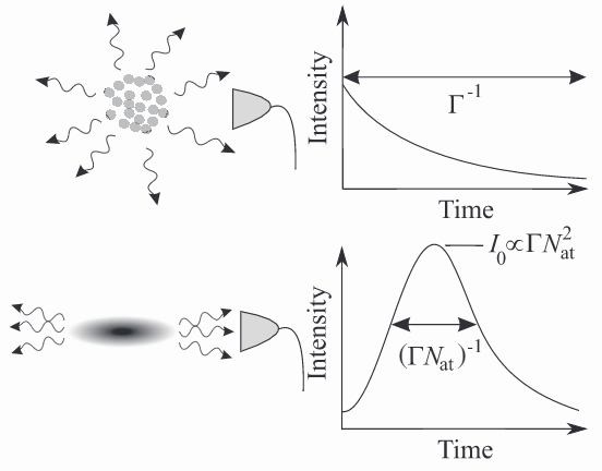
The quantum effect we are going to simulate is known as superradiance. It describes a phenomenon where, under certain conditions, independent light emitters (such as individual atoms) spontaneously build up quantum coherence and act cooperatively as a single entity. The coherence build-up causes the group to emit light in a single, high intensity burst. This burst is N times (!) stronger than the intensity expected from a group of independent particles, where N is the number of particles in the group. Interestingly, this effect is not based on any interaction between the particles but rather arises purely from symmetry properties of the particles’ interaction with the light field.

The following figure shows that light emission profiles are distinctly different for independent (upper panel) and superradiant (lower panel) particle ensembles. Superradiance causes a spatially directed, short time, and high intensity pulse as opposed to the classical exponentially decaying emission profile.

Superradiance has been observed or proposed in many different quantum systems. Let’s see how we can simulate superradiance from the nuclear spin ensemble of a Nitrogen-Vacancy Center in diamond using TensorFlow and Amazon SageMaker.

Anatomy of a scientific computation on Amazon SageMaker

The center point of a scientific computation on Amazon SageMaker is the notebook instance. From here, using Jupyter Notebooks, Amazon SageMaker helps you to orchestrate the different steps of a scientific workload (see the next figure):

Containerize your workload

Amazon SageMaker will send a Docker Image of your code and its dependencies (such as Python packages) to Amazon Elastic Container Service (ECS). Navigating to the Amazon ECS console in the AWS Management Console allows you to access and manage images you have sent in the past.

Define and spin up the compute environment

Amazon SageMaker will spin up a cluster of training instances and use the container that you have defined earlier in this blog post to run your computation. You can choose from a variety of instance types optimized for different workloads. By using multiple instances in your cluster, you can parallelize your computation if you need to.

Define input data and parameters of your workload

All input data that is required by your simulation can be stored in Amazon Simple Storage Service (S3). From there, Amazon SageMaker will transfer the data to a shared file system accessible for every instance of the cluster. Alternatively, you can stream the data directly from Amazon S3 using the Amazon SageMaker pipe mode. Besides using S3 to feed larger quantities of data, you can pass the parameters of your simulation directly to your container. We will see below how this works in practice.

Evaluate the results of your computation

After the computation is complete, Amazon SageMaker will write the results to an Amazon S3 location of your choice. The data can be retrieved from here and analyzed in the notebook.

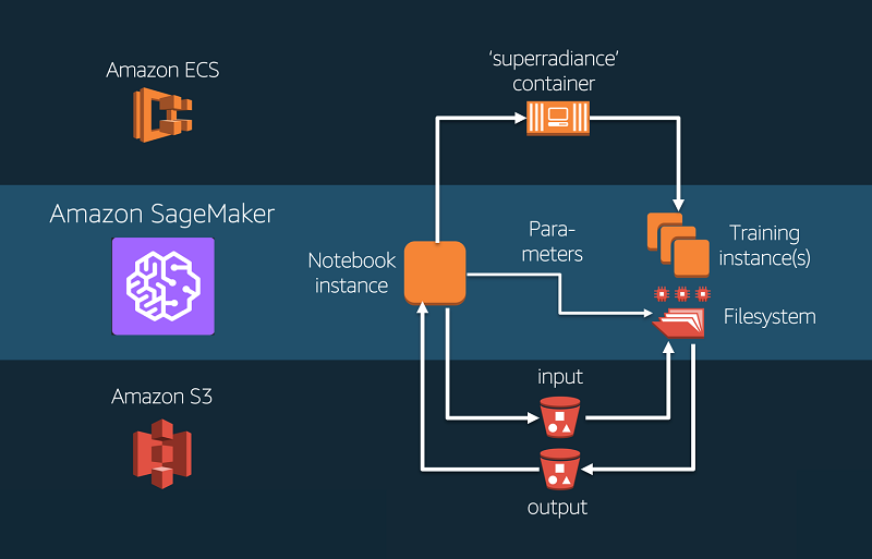
The following figure shows a workflow of a typical scientific computation on Amazon SageMaker. First Amazon SageMaker sends the containerized workload to a container registry on AWS. Then Amazon SageMaker spins up a cluster of one or more compute instances as specified by the user and loads the container image that holds the workload. Then input data and parameters are transferred from Amazon S3 to a shared file system accessible from all nodes in the cluster. After the computation is completed, the output is written to an Amazon S3 bucket from where it can be retrieved for further analysis in the notebook. All steps can be orchestrated from the Amazon SageMaker notebook instance.

Setup

To follow this example on your own AWS account, we need to go through a few steps to set up your environment.

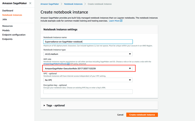
Step 0: Log into your AWS account and create a SageMaker notebook instance

Take note of the name of the IAM role you create in the process.

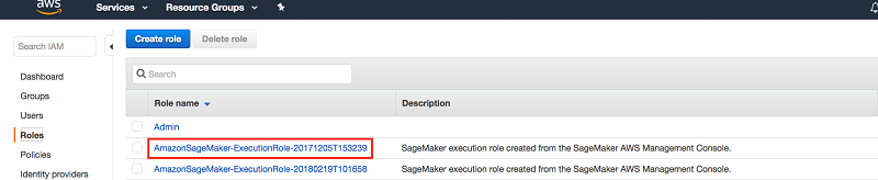
Step 1: Setting up permissions

Before getting started, we need to grant our SageMaker notebook instance additional permissions to access Amazon ECS. The easiest way to add these permissions is to add the managed policy to the role that you used to start your notebook instance in the SageMaker dashboard. To this end, navigate to the IAM console in your AWS Management Console, go to the Roles section, and find the SageMaker IAM role that you used to start your notebook instance in the Amazon SageMaker dashboard.

After you choose the role, you can attach the AmazonEC2ContainerRegistryFullAccess policy. There’s no need to restart your notebook instance when you do this, the new permissions will be available immediately.

Step 2: Load the code repo onto your SageMaker notebook instance

To follow through with this tutorial you also need to download the code repository onto your SageMaker notebook instance. It contains all the components you need to run a simulation on Amazon SageMaker and can be used as a template for your own use case.

First, open your SageMaker notebook from the Amazon SageMaker console.

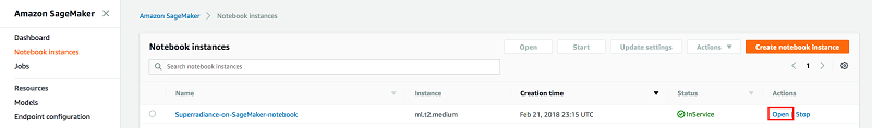
A new browser tab will open with the Jupyter file system. Log onto the server by opening a terminal session.

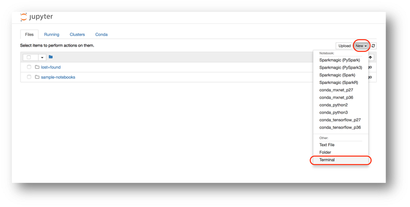
Use the following command in the terminal to download the code repository

git clone https://github.com/emkessler/sagemaker.git

The repo contains a container directory that has all the components you need to package the sample algorithm for Amazon SageMaker. You can find more information on the individual components in this SageMaker sample notebook. For our purpose, there are two files that are most relevant and contain all the information to run our workload.

Dockerfile describes how to build your Docker container image. Here you can define the dependencies of your code, e.g., which language you are using (Python), what packages your code needs (e.g., TensorFlow), and so on. Most of it is boilerplate and to adjust it to your use case typically requires changes to only a few lines. More details can be found here.

superradiance/train is the program that is invoked when the container is run for training. It takes a few parameters and the initial state of the system as input, runs a simulation of the system, and returns the light emission profile as a numpy array. For the moment, let’s not worry about how this simulation works. (You can find more details on the simulation in the Appendix.)

Step 3: Build and push the Docker image

To build the Docker image from the Dockerfile and push it to Amazon ECS we need to run the utility script build_and_push.sh. To this end, open the Jupyter notebook included in the repo and run the following in a cell:

import subprocess
print subprocess.check_output(['./build_and_push.sh', 'superradiance'])

The script will build a Docker image from the Dockerfile including the code in the superradiance directory and push it to the Amazon ECS repo with name superradiance (the argument passed to build_and_push.sh). If the Amazon -ECS repo doesn’t exist it will be created for you.

Now we are ready to execute our simulation on Amazon SageMaker.

Simulating superradiance on Amazon SageMaker

In this section, we are going to simulate superradiance from a so-called Nitrogen-Vacancy (NV) Center in diamond. An NV center is one of many possible defects of the carbon lattice that constitutes a diamond. Two carbon atoms are missing in the lattice, and in their place there is one nitrogen atom next to an empty spot. Have you ever seen a red diamond? Most likely, it had its color from an abundance of NV defects in the material. Besides giving diamonds a pretty color (that makes them VERY expensive), NV centers also happen to be excellent quantum systems. At the location of the defect, electrons can get trapped in a very stable fashion and researchers have mastered manipulating these electrons through laser light and microwave radiation. At the same time, the electrons interact through electromagnetic forces with the surrounding carbon atoms. Magnetic excitations of the carbon atoms can therefore travel through the electron and be emitted as photons from the NV center. Under the right conditions, this light emission can show signatures of superradiance.

Let’s get started by importing some modules and defining the parameters of the simulation, such as the number of time steps and carbon atoms we want to simulate.

from scipy import sparse
import numpy as np
import os
import pickle
import matplotlib.pyplot as plt

import boto3
from sagemaker import get_execution_role
import sagemaker as sage

steps = 500                  # Number of simulated time steps
N = 8                        # Number of nuclear spins
dim = 2**(N+1)               # Dimension of Hilbert space of N nuclear and 1 electronic spin

Let’s try out our simulation with 8 carbon atoms and 500 time steps. We will later pass these parameters to our program as hyperparameters.

Next, we define the initial state of the system. We will start our simulation from a simple initial state where at time t=0 all of the carbon atoms as well as the electrons are magnetically excited. In quantum mechanics, the state of such a composite system of atoms and electrons is represented by a 2D matrix, the so-called density matrix. Without going into detail about the mathematical formalism through which one can derive the matrix representation from a physical system, luckily, in our case the representation of the state is very simple. After we construct the state in the first three lines, we upload the resulting matrix to Amazon S3. The simulation will later retrieve this data to initialize the system.

# Define Nuclear and Electron spin states as density matrices
rhoI = sparse.csr_matrix(([1.],([0],[0])),shape =(int(dim/2),int(dim/2))) # All carbon atoms magnetically excited
rhoS = sparse.csr_matrix(([1.],([1],[1])),shape =(2,2))                   # Electron magnetically excited
sparse_rho =sparse.kron(rhoS, rhoI)                                       # Build the system density matrix

tempfile = '/tmp/tmp.pckl'
pickle.dump(sparse_rho, open(tempfile, "wb"))

# Upload serialized initial state to S3
resource = boto3.resource('s3') 
my_bucket = resource.Bucket('sagemaker-kessle31')                         #subsitute this for your s3 bucket name. 
my_bucket.upload_file(tempfile, Key='superradiance/initial_state/init.pckl')

# Clean up temporary files
os.remove(tempfile)

Now everything is ready to ship our simulation. After specifying the Docker image, we will create a training job that defines the hardware to be used for the simulation. Amazon SageMaker will then spin up the requested instances, pull the Docker image from Amazon ECS, and start the job. The program (as it is defined in the file superradiance/train) uses TensorFlow to solve the system of coupled differential equations that describes the system’s dynamics by sequential stepwise evolution.

role = get_execution_role()
sess = sage.Session()

# Specify the name of the ECS repo that contains your docker image. 
# By default the image with tag 'latest' in the repo will be utilized.
imagename = 'superradiance'  

account = sess.boto_session.client('sts').get_caller_identity()['Account']
region = sess.boto_session.region_name
image = '{}.dkr.ecr.{}.amazonaws.com/{}'.format(account, region, imagename)

# Define the training job
superradiance = sage.estimator.Estimator(image,
                       role, 1, 'ml.c4.2xlarge',
                       output_path="s3://sagemaker-kessle31/superradiance/output",
                       sagemaker_session=sess)

# Parameters can be passed to the simulation as a dictionary
superradiance.hyperparam_dict = {'N': N, 'steps': steps}

# Pass the location of the training data (see above) and start the job
superradiance.fit("s3://sagemaker-kessle31/superradiance/initial_state")
INFO:sagemaker:Creating training-job with name: superradiance-2018-02-22-16-31-48-732

The results of the simulation will be placed as a tar.gz file in the Amazon S3 location specified by the output_path argument. Let’s have a look at the results!

import tarfile

# get the results from S3
results = my_bucket.Object('superradiance/output/{}/output/model.tar.gz'.format(superradiance.latest_training_job.name))
tempfile = '/tmp/model.tar.gz'   
results.download_file('/tmp/model.tar.gz')    

# unzip the results
tar = tarfile.open(tempfile, "r:gz")
tar.extractall(path = '/tmp')

# load the results into the notebook
out = pickle.load(open('/tmp/out.pckl', "rb"))
intensity = out['intensity']
I_ind = out['I_ind']

# clean-up temporary files
os.remove(tempfile) 

# Vizualize the results
plt.scatter(range(steps-1),intensity/I_ind, label = 'Simulated System')
plt.scatter(range(steps-1), np.exp(-I_ind/N * np.arange(steps-1)), label = 'Classical System (benchmark)')
plt.xlabel('Time [a.u.]')
plt.ylabel('Intensity of emitted radiation [normalized]')
plt.legend()

plt.show()

The following figure shows the emission profile of the simulated particle ensemble (blue). The emission profile exhibits a strong burst of intensity when compared to the expected emission of a classical ensemble (orange).

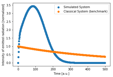
We can clearly see that the quantum system we have simulated exhibits a characteristic superradiance signature in the light emission profile (blue). As compared to the emission expected from an ensemble of classical particles (orange) the profile show a strong and distinct burst of radiation after a short time indicating superradiance.

Conclusion

In this blog post you have seen that besides streamlining the machine learning workflow, Amazon SageMaker can be used as a general purpose and fully managed compute environment. You have learned how you can use the Amazon SageMaker “bring your own algorithm” functionality to containerize a scientific workload, define data input and output channels, and execute the workload on a SageMaker cluster. You have seen that these tasks in the workflow of a scientific computation can all be orchestrated from a single hosted Jupyter notebook.

If you have questions or suggestions, please leave a comment.

Appendix: TensorFlow code that runs the simulation

The program that is executed (superradiance/train) in this blog post uses TensorFlow to solve the quantum master equation of the spin system by simple sequential stepwise evolution. The code, including explanations of the main steps, is replicated below:

!cat container/superradiance/train
#!/usr/bin/env python

# A sample program that simulates a simple quantum system exhibiting superradiance

from __future__ import print_function
import os
import json
import pickle
import sys
import traceback
import tensorflow as tf
import numpy as np
from utils import kronecker_product, SparseIndices               
from scipy import sparse                                          
import pandas as pd                                               

# These are the paths to where SageMaker mounts interesting things in your container.

prefix = '/opt/ml/'

input_path = prefix + 'input/data'

output_path = os.path.join(prefix, 'output')                       # Failure output & error messages should be written here
model_path = os.path.join(prefix, 'model')                         # All results should be written here 
param_path = os.path.join(prefix, 
                          'input/config/hyperparameters.json')     # Passed parameters can be retrieved here

# This algorithm has a single channel of input data called 'training'. Since we run in
# File mode, the input files are copied to the directory specified here.
channel_name='training'
training_path = os.path.join(input_path, channel_name)              # The initial state is found here 



# The function to execute the training.
def train():
    print('Starting the training.')
    try:        
        ##################################################################################
        # Retrieve parameters
        ##################################################################################
        # Parameters that were defined in the hyperparameter dict in the notebook 
        # (in our example: superradiance.hyperparam_dict = {'N': N, 'steps': steps})  
        # can be retrieved from the param_path defined above. 
        # Note that the parameters are stored as a JSON string, so it is required to 
        # define the correct dtype upon reading (here: int).
        
        datatype = tf.complex128
        
        with open(param_path, 'r') as tc: 
             trainingParams = json.load(tc)
        N = int(trainingParams.get('N', None))          # Number of simulated nuclear spins as defined in notebook
        steps = int(trainingParams.get('steps', None))  # Number of simulated time steps

        dim = 2**(N+1)                                  # Dimension of Hilbert space of N nuclear and 1 electronic spin
        
        #################################################################################
        # Define some other parameters
        ##################################################################################
        
        Amean = 1
        gamma = 1
        #g = np.random.randn(N) 
        g = np.ones(N)
        g = g/(np.sqrt((g**2).sum()))                    # Coupling strengts
        A = Amean/g.sum()
        I_ind = np.real(A**2/(gamma+1j*Amean))*2/N       # Classical emission intensity of N independent emitters (benchmark)        
        
        ##################################################################################
        # Define TF constants
        ##################################################################################
        
        gammaT = tf.constant(gamma, dtype=datatype)
        AT = tf.constant(A, dtype=datatype)
        eps = tf.placeholder(dtype=datatype, shape=())

        ##################################################################################
        # Define 'Pauli Matrices'
        ##################################################################################
        # The most elemental quantum mechanical spins system is a spin-1/2. It can be 
        # represented through three simple matrices, called Pauli Matrices. For more 
        # information, there are many great online resources, e.g., 
        # http://galileo.phys.virginia.edu/~pf7a/msm3.pdf

        sigmaz = tf.constant([[1/2, 0], [0, -1/2]], dtype= datatype)
        splus  = tf.constant([[0, 1], [0, 0]], dtype = datatype)
        sminus = tf.constant([[0, 0], [1, 0]], dtype = datatype)

        ##################################################################################
        # Electron Spin operators 
        ##################################################################################
        # States of a quantum system live in a vector space with special properties, 
        # called the Hilbert space. 
        # The Hilbert space of a composite system of multiple spins can be constructed by
        # taking the tensor product of the individual 1-particle spaces. 
        # Using this property, it can be shown that we can construct the multi-spin 
        # operators by taking the the Kronecker product (https://en.wikipedia.org/wiki/Kronecker_product)
        # of the individual spin operators with the identity matrix of appropriate dimension 
        # (see, section 3.2 of http://galileo.phys.virginia.edu/~pf7a/msm3.pdf)
        # Let's see how that looks like for our electron operator:

        Sm = kronecker_product(sminus, tf.eye(int(dim/2), dtype = datatype))
        Sp = tf.transpose(Sm)
        Sz = kronecker_product(sigmaz, tf.eye(int(dim/2), dtype = datatype))

        ##################################################################################
        # Nuclear Spin operators 
        ##################################################################################
        # Similarly to the case of the electron operator, we create one spin operator 
        # for every nuclear spin we simulate, and take the sum over all nuclear operators 
        # (because the electron interacts with all of them)

        Am = tf.zeros(int(dim/2), dtype = datatype)
        Iz = tf.zeros(int(dim/2), dtype = datatype)
        for p in range(N): 
            Am = Am + g[p]*kronecker_product(kronecker_product(tf.eye(2**p, dtype = datatype),sminus)
                                           ,tf.eye(2**(N-1-p), dtype = datatype))
            Iz = Iz +      kronecker_product(kronecker_product(tf.eye(2**p, dtype = datatype),sigmaz)
                                           ,tf.eye(2**(N-1-p), dtype = datatype))

        Am = kronecker_product(tf.eye(2, dtype = datatype),Am)
        Ap = tf.transpose(Am)
        Iz = kronecker_product(tf.eye(2, dtype = datatype),Iz)
            
        ##################################################################################
        # Load and construct Initial State
        ##################################################################################
        # You can pass on larger data structures to your program by placing them on S3 and 
        # and point to the location at execution time.
        # (in our example: superradiance.fit("s3://sagemaker-kessle31/superradiance/initial_state")
        # It can be retrieved from the 'training_path' location defined above.           
            
        sparse_rho = pickle.load(open(os.path.join(training_path, 'init.pckl'), "rb"))

        rho_ind = SparseIndices(sparse_rho)
        rho2 = tf.sparse_to_dense(rho_ind['indices'], 
                                  rho_ind['dense_shape'], 
                                  rho_ind['values'])         # Sparse_to_dense not implemented for complex at time of this 
                                                             # notebook => Construct Real an Imag separately
        rho1 = tf.complex(rho2,tf.zeros(rho_ind['dense_shape'], dtype=tf.float64))
        rho = tf.Variable(rho1, dtype=datatype)  

        ##################################################################################
        # Define Operations
        ##################################################################################
        # The Hamiltonian and Lagrangian are operators codifying the dynamics and interactions 
        # of a Quantum System.
        # The system we are simulating is a simple central spin system represented by the 
        # following Hamiltonian/Lagrangian:
        # (https://journals.aps.org/prl/abstract/10.1103/PhysRevLett.104.143601)  
        
        H = 0.5 * AT * (tf.matmul(Sp,Am) + tf.matmul(Sm,Ap))  # Define the Hamiltonian of the system
        
        IL = gammaT*(tf.matmul(tf.matmul(Sm,rho),Sp) 
                     - 0.5 * (tf.matmul(tf.matmul(Sp,Sm),rho) 
                              + tf.matmul(rho, tf.matmul(Sp,Sm))))\
              - 1j * (tf.matmul(H,rho) - tf.matmul(rho, H))   # Define the Lagrangian of the system
            
        rho_ = rho + eps * IL                                 # Evolve the system by one time step
        
        pol = tf.real(tf.trace(tf.matmul(rho, Iz)))           # Compute the polarization of the nuclear system,

        global_step = tf.train.get_or_create_global_step()
        increment_global_step_op = tf.assign(global_step, global_step+1)
        
        step = tf.group(rho.assign(rho_),increment_global_step_op) 
        
        ##################################################################################
        # Run the Simulation     
        ##################################################################################
        
        polarization = np.zeros(steps)        
        init = tf.global_variables_initializer()
        with tf.Session() as sess:
            sess.run(init)            
            for i in range(steps):
                _ , polarization[i] = sess.run([step, pol], feed_dict={eps:0.3})
                
        ##################################################################################
        # Compute output and dump to pickle                       
        ##################################################################################                       
        # Everything written into the 'model_path' location defined above will be
        # returned by SageMaker to the S3 location defined in the notebook 
        # (in our example: output_path="s3://sagemaker-kessle31/superradiance/output")
        # Note that the files will be returned as a tar.gz archive       
        
        intensity = -np.diff(polarization)                                  
        out= {'intensity': intensity, 'I_ind': I_ind}
        pickle.dump(out, open(os.path.join(model_path, 'out.pckl'), "wb"))
        
        print('Training complete.')
        
    except Exception as e:
        # Write out an error file. This will be returned as the failureReason in the
        # DescribeTrainingJob result.
        trc = traceback.format_exc()
        with open(os.path.join(output_path, 'failure'), 'w') as s:
            s.write('Exception during training: ' + str(e) + '\n' + trc)
        # Printing this causes the exception to be in the training job logs, as well.
        print('Exception during training: ' + str(e) + '\n' + trc, file=sys.stderr)
        # A non-zero exit code causes the training job to be marked as Failed.
        sys.exit(255)

if __name__ == '__main__':
    train()

    # A zero exit code causes the job to be marked a Succeeded.
    sys.exit(0)

About the Author

Eric Kessler is a Data Scientist with AWS Professional Services. He has a PhD from the Max-Planck Institute for Quantum Optics in Germany and has worked multiple years as an academic researcher in quantum physics. Today he is working with customers to develop and integrate machine learning and AI solutions on AWS.