AWS Public Sector Blog
Decrease geospatial query latency from minutes to seconds using Zarr on Amazon S3
Geospatial data, including many climate and weather datasets, are often released by government and nonprofit organizations in compressed file formats such as the Network Common Data Form (NetCDF) or GRIdded Binary (GRIB). Many of these formats were designed in a pre-cloud world for users to download whole files for analysis on a local machine. As the complexity and size of geospatial datasets continue to grow, it is more time- and cost-efficient to leave the files in one place, virtually query the data, and download only the subset that is needed locally.
Unlike legacy file formats, the cloud-native Zarr format is designed for virtual and efficient access to compressed chunks of data saved in a central location such as Amazon Simple Storage Service (Amazon S3) from Amazon Web Services (AWS).
In this walkthrough, learn how to convert NetCDF datasets to Zarr using an Amazon SageMaker notebook and an AWS Fargate cluster and query the resulting Zarr store, reducing the time required for time series queries from minutes to seconds.
Legacy geospatial data formats
Geospatial raster data files associate data points with cells in a latitude-longitude grid. At a minimum, this type of data is two-dimensional but grows to N-dimensional if, for example, multiple data variables are associated with each cell (for example, temperature and windspeed) or variables are recorded over time or with an additional dimension such as altitude.
Over the years, a number of file formats have been devised to store this type of data. The GRIB format created in 1985 stores data as a collection of compressed two-dimensional records, with each record corresponding to a single time step. However, GRIB files do not contain metadata that supports accessing records directly; retrieving a time series for a single variable requires sequential access to every single record.
NetCDF was introduced in 1990 and improved on some of the shortcomings of GRIB. NetCDF files contain metadata that supports more efficient data indexing and retrieval, including opening files remotely and virtually browsing their structure without loading everything into memory. NetCDF data can be stored as chunks within a file, enabling parallel reads and writes on different chunks. As of 2002, NetCDF4 uses the Hierarchical Data Format version 5 (HDF5) as a backend, improving the speed of parallel I/O on chunks. However, the query performance of NetCDF4 datasets can still be limited by the fact that multiple chunks are contained within a single file.
Cloud-native geospatial data with Zarr
The Zarr file format organizes N-dimensional data as a hierarchy of groups (datasets) and arrays (variables within a dataset). Each array’s data is stored as a set of compressed, binary chunks, and each chunk is written to its own file.
Using Zarr with Amazon S3 enables chunk access with millisecond latency. Chunk reads and writes can run in parallel and be scaled as needed, either via multiple threads or processes from a single machine or from distributed compute resources such as containers running in Amazon Elastic Container Service (Amazon ECS). Storing Zarr data in Amazon S3 and applying distributed compute not only avoids data download time and costs but is often the only option for analyzing geospatial data that is too large to fit into the RAM or on the disk of a single machine.
Finally, the Zarr format includes accessible metadata that allows users to remotely open and browse datasets and download only the subset of data they need locally, such as the output of an analysis. The figure below shows an example of metadata files and chunks included in a Zarr group containing one array.
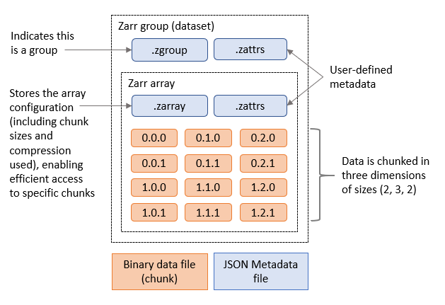
Figure 1. Zarr group containing one Zarr array.
Zarr is tightly integrated with other Python libraries in the open-source Pangeo technology stack for analyzing scientific data, such as Dask for coordinating distributed, parallel compute jobs and xarray as a an interface for working with labeled, N-dimensional array data.
Zarr performance benefits
The Registry of Open Data on AWS contains both NetCDF and Zarr versions of many widely-used geospatial datasets, including the ECMWF Reanalysis v5 (ERA5) dataset. ERA5 contains hourly air pressure, windspeed, and air temperature data at multiple altitudes on a 31 km latitude-longitude grid, since 2008. We compared the average time to query one, five, nine, and 13 years of historical data for these three variables, at a given latitude and longitude, from both the NetCDF and Zarr versions of ERA5.
| Length of time series | Avg. NetCDF query time (seconds) | Avg. Zarr query time (seconds) |
| 1 year | 23.8 | 1.3 |
| 5 years | 82.7 | 2.4 |
| 9 years | 135.8 | 3.5 |
| 13 years | 193.1 | 4.7 |
Figure 2. Comparison of the average time to query three ERA5 variables using a Dask cluster with 10 workers (8 vCPU, 16 GM memory.
Note that these tests are not a true one-to-one comparison of file formats since the size of the chunks used by each format differs, and results can also vary depending on network conditions. However, they are in line with benchmark studies that show a significant performance advantage for Zarr compared to NetCDF.
While the Registry of Open Data on AWS contains Zarr versions of many popular geospatial datasets, the Zarr chunking strategy of those datasets may not be optimized for an organization’s data access patterns, or organizations may have substantial internal datasets in NetCDF format. In these cases, they may wish to convert from NetCDF files to Zarr.
Moving to Zarr
There are several options for converting NetCDF files to Zarr: a Pangeo-forge recipe, using the Python rechunker library, and using xarray.
The Pangeo-forge project provides premade recipes that may enable you to convert some GRIB or NetCDF datasets to Zarr without diving into the low-level details of the specific formats.
For more control of the conversion process, you can use the rechunker and xarray libraries. Rechunker enables efficient manipulation of chunked arrays saved in persistent storage. Because rechunker uses an intermediate file store and is designed for parallel execution, it is useful for converting datasets larger than working memory from one file format to another (such as from NetCDF to Zarr), while simultaneously changing the underlying chunk sizes. This makes it ideal for converting large NetCDF datasets to an optimized Zarr format. Xarray is useful for converting smaller datasets to Zarr or appending data from NetCDF files to an existing Zarr store, such as additional data points in a time series (which rechunker currently does not support).
Finally, while technically not an option for converting from NetCDF to Zarr, the Kerchunk python library creates index files that allow a NetCDF dataset to be accessed as if it is a Zarr store, yielding significant performance improvements relative to NetCDF alone without creating a new Zarr dataset.
The rest of this blog post provides step-by-step instructions for using rechunker and xarray to convert a NetCDF dataset to Zarr.
Overview of solution
This solution is deployed within an Amazon Virtual Private Cloud (Amazon VPC) with an internet gateway attached. Within the private subnet, it deploys both a Dask cluster running on AWS Fargate and the Amazon SageMaker notebook instance that will be used to submit jobs to the Dask cluster. In the public subnet, a NAT Gateway provides internet access for connections from the Dask cluster or the notebook instance (for example, when installing libraries). Finally, a Network Load Balancer (NLB) enables access to the Dask dashboard for monitoring the progress of Dask jobs. Resources within the VPC access Amazon S3 via an Amazon S3 VPC Endpoint.
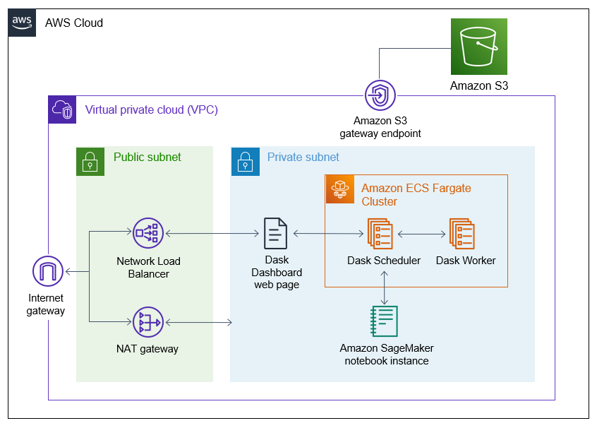
Figure 3. Architecture diagram of the solution.
Solution walkthrough
The following is a high-level overview of the steps required to perform this walkthrough, which we present in more detail:
- Clone the GitHub repository.
- Deploy the infrastructure using the AWS Cloud Development Kit (AWS CDK).
- (Optional) Enable the Dask dashboard.
- Set up the Jupyter notebook on the SageMaker notebook instance.
- Use the Jupyter notebook to convert NetCDF files to Zarr.
The first four steps are mostly automated and should take roughly 45 minutes. Once that setup is complete, it should take 30 mins to run the cells in the Jupyter notebook.
Prerequisites
Before starting this walkthrough, you should have the following prerequisites:
- An AWS account
- AWS Identity and Access Management (IAM) permissions to follow all of the steps in this guide
- Python3 and the AWS CDK installed on the computer you will deploy the solution from.
Deploying the solution
Step 1: Clone the GitHub repository
In a terminal, run the following code to clone the GitHub repository containing the solution.


