Getting started with Amazon Lightsail for Research: A tutorial using RStudio

Amazon Lightsail for Research is a new service from Amazon Web Services (AWS) that makes it simple to incorporate cloud computing resources into your work without cloud experience. With Lightsail for Research, you can shift large and/or time-consuming analysis from your laptop onto powerful cloud resources, run multiple analyses simultaneously, and continue computations even when your laptop is off or being used for other activities. By accessing research-class computing power along with pre-installed research software, you can get to work quickly without having to set up computers, install software, or find someone to perform those tasks — all without having to understand cloud infrastructure.

With its emphasis on simplicity, Lightsail for Research offers straightforward pricing that bundles everything you need into a single number, making it simple to understand spending before you start working. Lightsail for Research supports cost control rules by automatically shutting down a virtual computer when a rule detects that the resource is not being used. For example, if your analysis finishes in the middle of the night, or you simply get busy and forget, cost control rules can keep you from spending unnecessarily. When you have completed your work, and after you have retrieved your results, resources can be deleted as simply as they were created, realizing one of the best features of the cloud: elasticity.

In this blog post, we walk through Lightsail for Research with a simple but common use case.

Solution overview: Setting up Lightsail for Research with RStudio

In this walkthrough, we use RStudio, a popular data analysis and machine learning (ML) integrated development environment, to analyze global weather data using the National Oceanic and Atmospheric Administration’s (NOAA) Global Surface Summary of the Day dataset. This data offers various daily weather measurements from over 9,000 weather stations around the world, some going back to 1929. It is a reasonably large dataset at 37GB made up of over 550K files. As this is not a tutorial about using R or weather data, we keep the analysis straightforward by asking a simple question: What are the maximum median surface temperatures recorded by year from 1929 through 2022?

Prerequisites

To get started, you need an AWS Account. Sign up here or speak to your institution for how best to access AWS. Amazon Lightsail for Research is AWS Free Tier eligible.
Following this tutorial will take approximately 15 minutes of your time and 2.5 hours for all steps to complete.

Deploying the solution

Create a virtual computer

To perform the analysis, first create a Lightsail for Research virtual computer. In your AWS account, navigate to the Lightsail for Research console. Once logged in, select an AWS Region geographically closest to you. An AWS Region indicates where the virtual computer resources you create will be physically located. Then, in the application section, choose RStudio (Figure 1).

Figure 1. The getting started wizard for Lightsail for Research. Select an AWS Region near your physical location, then choose RStudio from the list of offered applications.

Next, we see a selection of hardware bundles to power the virtual computer. The bundles can be understood as offering different amounts of processing power in the form of CPU cores, memory, and GPU. For this tutorial, we select the Standard XL bundle for our analysis; because the computational needs are small, we only compute a maximum value and evaluating a year’s worth of data at a time, which uses significantly less than 8GB of memory.

Once you select a bundle, give the virtual computer a name in the Name your virtual computer field; you may need to scroll down to see it. For this walkthrough, we name it noaa-gsod-analysis. It is a best practice to name your virtual computer something that indicates what you are doing with it. Finally, select the orange Create virtual computer button to start the process of provisioning your virtual computer (Figure 2).

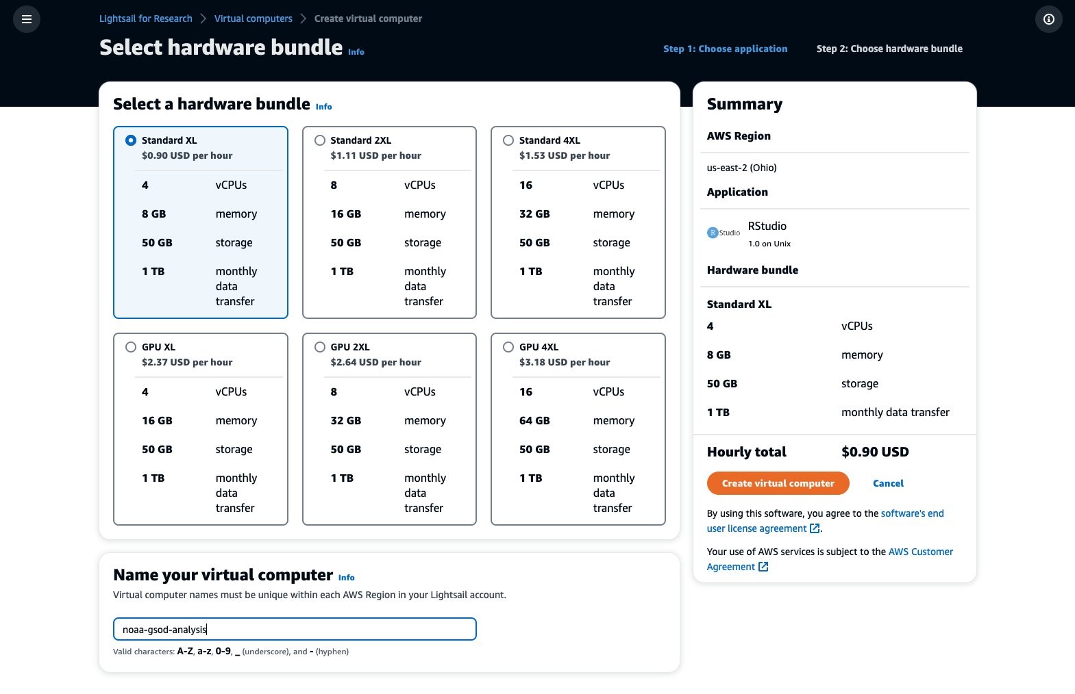
Figure 2. The select hardware bundle wizard for Lightsail for Research. Select a hardware bundle, name your virtual computer, and choose the create virtual computer button.

It may take up to a couple of minutes for the virtual computer to be provisioned and start up. You can watch its progress within the virtual computer’s tile on the virtual computer’s summary page (Figure 3). Once the process completes, a confirmation banner appears at the top of the page, and a green “Running” indicator appears on the upper-right corner of the tile. Next, examine the details of the virtual computer by choosing the virtual computer’s name in the summary tile.

Figure 3. Virtual computers summary in Lightsail for Research. Virtual computer tile(s) indicate status (e.g. running/stopped) and provide controls to start/stop computer and launch an application (e.g. RStudio).

Create a cost control rule

The virtual computer detail page displays its status and configuration, an application launch button, usage summary, CPU statistics, and cost control rules (Figure 4). In the Cost control rules panel, choose Manage in cost control.

Figure 4. Virtual computer detail in Lightsail for Research.

Cost control rules enable virtual computers to automatically turn off when the rule’s conditions are met. The available rule can stop a virtual computer when it’s been idle for a period of time. When a virtual computer is stopped, spending is reduced significantly as it accrues only a very small charge to maintain its system disk. To configure a cost control rule, choose the orange Create rule button.

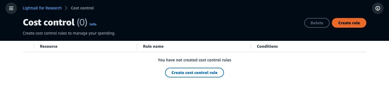
Figure 5. Cost control management in Lightsail for Research. At first, no cost controls rules are defined.

The Create rule wizard (Figure 6) asks for which resource the new rule will apply to. Currently, the only resources that Lightsail for Research offers cost control rules for are virtual computer resources. In the Select resource field, make sure your virtual computer is selected. The Stop virtual computer settings section allows us to set a threshold which defines a CPU utilization below which the rule considers the virtual computer to be idle. In this walkthrough, we use the default threshold of 5%. You can also set a time period, which is the amount of time the virtual computer must remain idle, below 5% utilized, before the rule stops the virtual computer. In this tutorial, we use the default time period of ten minutes. So, if the CPU utilization remains below 5% for ten minutes, the rule will stop the virtual computer automatically. Choose the orange Create rule button to put the rule into effect.

Figure 6. The cost control create rule wizard in Lightsail for Research.

The wizard next asks to confirm the rule’s settings. Pay particular attention to the warning: if you enable a cost control rule, you need to make sure you are saving your work, as Lightsail for Research will not do it for you. Choose the orange Confirm button to enable the rule on the noaa-gsod-analysis virtual computer (Figure 7).

Figure 7. The cost control rule enablement confirmation in Lightsail for Research.

On the Cost control page, a cost control rule is now defined (Figure 8). Navigate to the virtual computer detail page by choosing its name from the menu on the left. If the menu is not visible, choose the hamburger icon (three horizontal lines) in the upper left to display it.

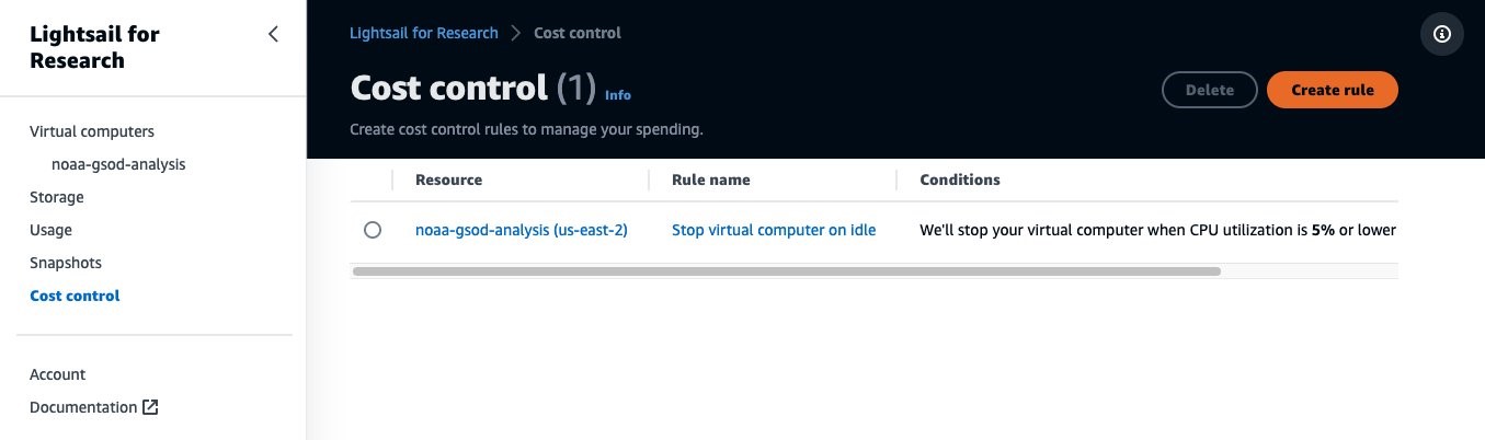
Figure 8. The cost control management in Lightsail for Research. One cost control rule defined.

Create a data disk

On the Virtual computer detail page, add storage to hold the analysis data by choosing the Storage tab. There’s already a 50GB system disk (Figure 9), which is used primarily for the operating system and applications. You could use the system disk for data, but a better practice is to put data on its own storage to keep from both filling up and cluttering the system disk. To prepare for that, choose the Create disk button in the disks section.

Figure 9. Virtual computer storage detail in Lightsail for Research. Disk status details include name, size, disk mount status, disk path, and date created along with buttons to create and attach/detach disks.

The Create disk wizard (Figure 10) prompts to select a size for the disk and give it a name. For this tutorial, we pick 64GB, as that is large enough to hold the data we need for our analysis (37GB.) Name the disk something meaningful to the disk once it is attached to the virtual computer; in this example, we use noaa-gsod. To create the disk, choose the orange Create disk button. You can think of this step as similar to acquiring an external disk for your laptop.

Figure 10. Create disk wizard in Lightsail for Research. Select a region, choose your disk size, name your disk, and choose the create disk button.

Once the disk is created, it will be confirmed by a banner at the top of the next screen. Now, attach the new disk to the virtual computer. Choose the virtual computer noaa-gsod-analysis in the drop-down menu and choose the orange Attach disk button (Figure 11). You can think of this step as similar to plugging an external disk into your laptop.

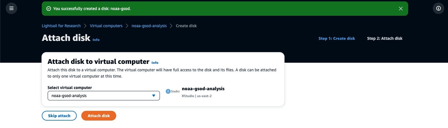
Figure 11. Attach disk wizard in Lightsail for Research. Select virtual computer to attach disk to and choose the attach disk button.

Return to the Virtual computer detail dashboard. From there, select the Storage tab. The new disk appears in the disks section and its mount status transitions to “Mounted” in green. Mounted means the disk is attached to the virtual computer and is now ready to use (Figure 12).

Figure 12. Virtual computer storage detail in Lightsail for Research. Disk status showing newly created disk has a disk mount status of “mounted.”

With the disk attached, the virtual computer is fully configured. To start RStudio, select the dashboard tab and choose the Launch RStudio button (Figure 13). Alternatively, launch RStudio directly from the system’s tile on the virtual computer’s summary page.

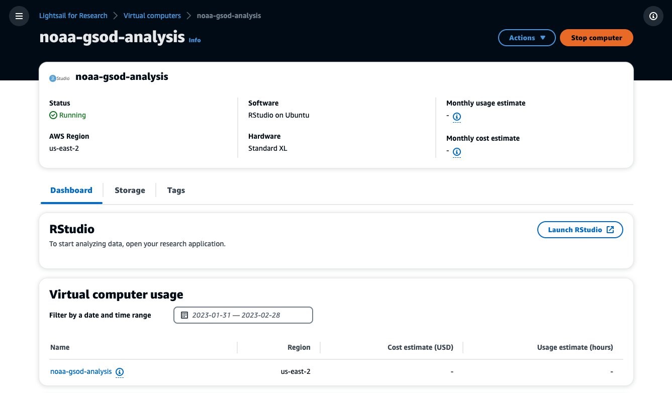
Figure 13. Virtual computer dashboard detail in Lightsail for Research.

During the launch (Figure 14), a spinning indicator and progress bar advance as the virtual computer and RStudio start up.

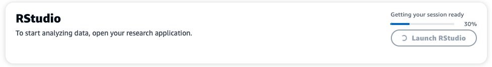
Figure 14. Virtual computer detail dashboard in Lightsail for Research. Close up of RStudio launching.

Analysis

A short while later, a new browser tab will automatically open. If not, check your browser’s pop-up blocker. The new tab connects directly to the RStudio application session (Figure 15). A session is what connects users visually to the virtual computer and application. The whole process—from selecting an application and hardware bundle, to creating and attaching a disk, to it all being ready to use—takes only minutes.

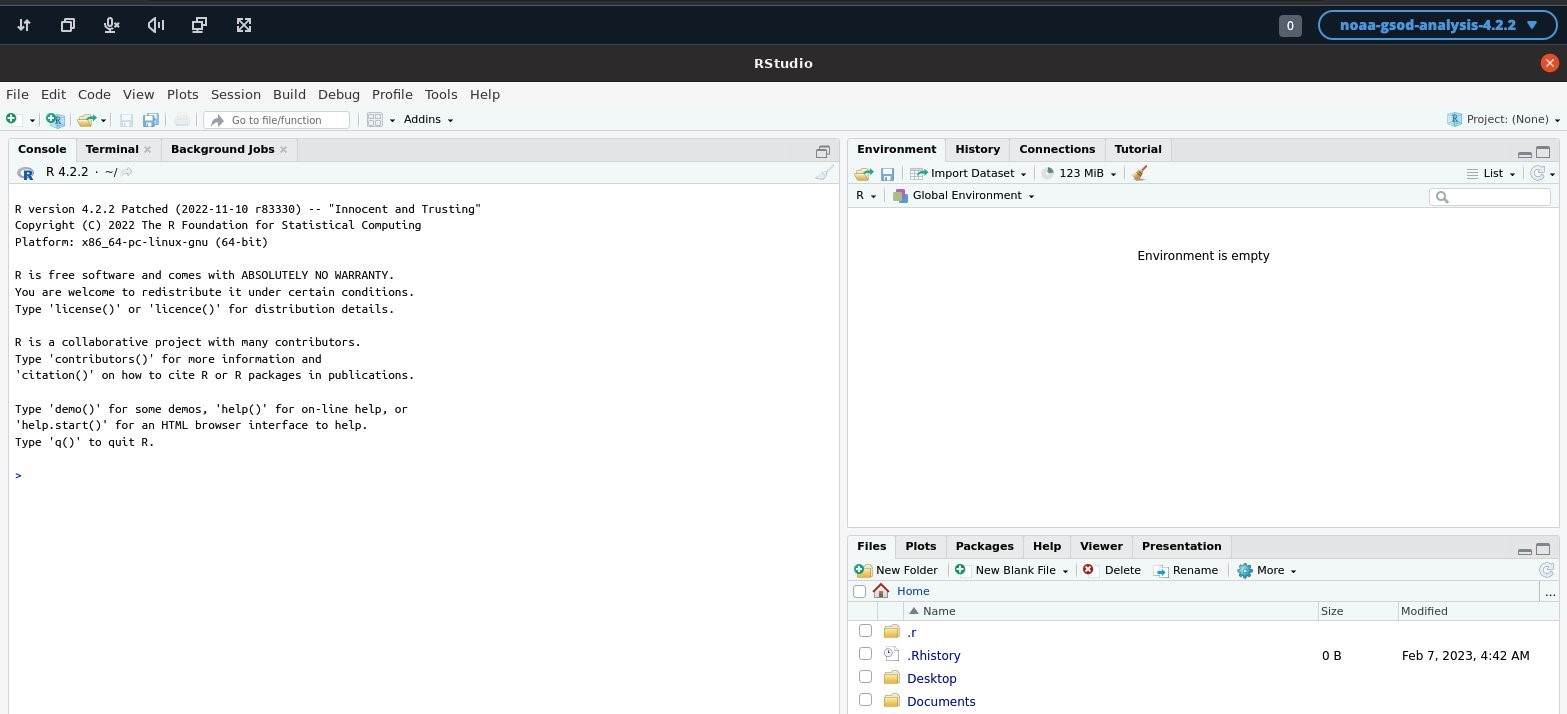
Figure 15. A virtual computer application session connected to RStudio.

Choose the Terminal tab inside RStudio. Type in the command ls and press the enter/return key on your computer. Review the output and notice that the disk you created, attached, and mounted—noaa-gsod—appears in the listing, ready to use for storing data (Figure 16). Leave the RStudio terminal open for the first step in the analysis by downloading the dataset.

Figure 16. RStudio terminal showing that our disk, noaa-gsod, is connected and ready to use.

Download the data from the Registry of Open Data on AWS

Download the NOAA Global Surface Summary of the Day data from the Registry of Open Data on AWS to the virtual computer. You can download the dataset using AWS Command Line Interface (AWS CLI) by entering the following command into the RStudio terminal tab. The command copies the dataset from an Amazon Simple Storage Service (Amazon S3) bucket within the Registry of Open Data on AWS to the folder named noaa-gsod on the virtual computer, which is how you can access and make use of the disk storage created previously.

aws s3 cp --no-sign-request s3://noaa-gsod-pds/ noaa-gsod/ --recursive

The copy command above starts immediately and takes about 90 minutes to complete. For comparison, when we downloaded the data using a plugged-in, modern laptop with excellent WiFi and internet connection, the download took about 2.5 hours. During that time, the laptop could not be used for much else without extending the download even longer. In our walkthrough, the Lightsail for Research virtual computer downloaded the data in 40% less time than the laptop. Meanwhile, the laptop was no longer preoccupied with downloading data for 2.5 hours. In fact, you can shut-off your laptop immediately after entering the command above and the download will continue on the Lightsail for Research virtual computer in the cloud.

Cost management rule

Stepping away from our virtual computer while the download proceeds to spend time on something more productive is a reasonable thing to do. Lightsail for Research’s cost control feature helps us feel less anxiety about doing so. The rule we created earlier should stop our virtual computer after the download completes and the virtual computer’s CPU utilization drops to idle. When the CPU utilization stays below the 5% threshold for ten minutes, that condition will trigger the rule to stop the virtual computer for us automatically. You can test the rule by examining the browser tab containing the application session used earlier. In our walkthrough, we see that the session has been closed (Figure 17). This is a clue that the virtual computer has indeed been stopped. All the data we just copied is safe, stored on our disk, and not affected by stopping the virtual computer.

Figure 17. Terminated virtual computer application session message.

Remove the browser tab with the closed application session and switch to the browser tab containing the Lightsail for Research console. Log back into AWS, if necessary, and navigate back to the Lightsail for Research console. The virtual computer should be in the stopped state (Figure 18). Restarting RStudio is as simple as choosing Start computer and then, once the virtual computer is running, choosing the Launch RStudio button, which in turn starts the virtual computer and application session again.

Figure 18. Virtual computers summary page in Lightsail for Research. Showing the noaa-gsod virtual computer is in the stopped state due to a cost control rule.

Analyze the data using RStudio

With the data previously downloaded onto the noaa-gsod disk, we start our analysis. The R script below can be copied and pasted into the RStudio script editor tab. The script reads in data one year at a time and finds the maximum, median surface temperature for each year in the dataset, prints the result for each year to the RStudio console, and plots the full results at the end.

This is a good point to revisit what happens when a cost control rule’s parameters are satisfied and a virtual computer is stopped. When creating the cost control rule earlier, a warning states that any unsaved data will be lost. To not lose the results of the analysis, make sure to include code to save the plot to disk as a PDF. That way, if you step away from our session, and the analysis completes, and the cost control rule stops our virtual computer, the results save to the disk and you can still retrieve the plot.

setwd( "~/noaa-gsod" )
data_years = data.frame( matrix( ncol = 2, nrow = 0 ) )
colnames( data_years ) = c( "Year", "Temp" )
for ( yr in 1929:2022 ) {
    data_files = list.files( as.character( yr ), full.names = TRUE )
    data = do.call( rbind, lapply( data_files, function( f ) { read.csv( f, na.strings = c( 9999.9 ) ) } ) )
    max_median = max( data$TEMP, na.rm = TRUE )
    data_years[ nrow( data_years ) + 1, ] = c( yr, max_median )
   message( yr, " : ", max_median )
}
# save plot to disk
pdf("max_med_temp.pdf")
plot( data_years$Year, data_years$Temp, xlab = "Year", ylab = "Temperature (degrees F)", ylim = c( 80, 120 ), main = "Maximum Median Temperature (degrees F)" )
dev.off()

For our walkthrough, executing this R script on our virtual computer took about 40 minutes to complete. Executing the same R script on a modern laptop can take about the same length of time. The speed in both cases is ultimately limited by disk throughput on both systems given the large number of files processed (>550K). If you walked away during the analysis, you may come back to find the virtual computer stopped. This is because the cost control rule will have triggered again after the analysis completes. Simply starting the virtual computer and launching RStudio again will re-instate the application session in a new browser tab. Once the session is active, you can download the resulting plot to your laptop. To do that, choose the black and white up and down arrow icon located in the upper left corner of the browser tab (Figure 19).

Figure 19. Detail of the upper left corner of the RStudio session in Lightsail for Research. The black and white icons are remote session controls.

A dialog box appears showing the virtual computer’s file system. Find the data disk folder noaa-gsod and choose it. Then, using the paging controls (< and >), step through the folder for the analysis output file, max_med_temp.pdf, choose it, and choose the Actions drop down menu, then choose the Download menu item (Figure 20).

Figure 20. Download dialog of the RStudio session in Lightsail for Research. It displays a list of files on the virtual computer.

Opening the downloaded file max_med_temp.pdf locally on a laptop reveals the results of the analysis — a plot of the maximum, median temperatures from the NOAA Global Surface Summary of the Day (Figure 21). The reason the data before about 1970 looks so scattered is that there were many fewer stations reporting data around the world at the time. By the early seventies, there were enough for the results to stabilize.

Figure 21. Maximum median temperature from 1929-2022 plot from the NOAA Global Surface Summary of Day dataset.

Cleaning up

Deleting the virtual computer and storage resources are just as simple as creating them. A virtual computer can be deleted by choosing the actions menu (little arrow inside of a circle) on the right side of its summary tile (Figure 20). Choosing Delete virtual computer begins the process.

Figure 22. Lightsail for Research virtual computers summary page. Choosing the virtual computer noaa-gsod-analysis action menu reveals the delete virtual computer option.

Before the virtual computer is deleted, a warning dialog box appears and requires confirmation of the action. Enter the word “Confirm” and choose the orange Delete virtual computer button (Figure 23).

Figure 23. Lightsail for Research delete virtual computer confirmation dialog box.

While the virtual computer has now been permanently deleted, the data disk has not. Lightsail for Research does not presume you want to delete both because there may be circumstances where the data on it and/or the storage could be reused with a future virtual computer. To proceed with deleting the disk noaa-gsod, choose Storage from the menu on the left. If the menu is not visible, choose the hamburger icon (three horizontal lines) in the upper left to display it (Figure 22).

Figure 24. Lightsail for Research virtual computers summary page. A green banner confirms the virtual computer noaa-gsod-analysis has been deleted.

On the storage summary page, first choose the noaa-gsod disk, followed by choosing the Delete disk button (Figure 25).

Figure 25. Lightsail for Research storage summary page. Selecting the disk enables the delete disk button.

Similar to the virtual computer delete process, a warning dialog box requires confirmation of the action. Enter the word “confirm” and choose the orange Delete button (Figure 26).

Figure 26. Lightsail for Research disk delete confirmation dialog box.

Conclusion

This walkthrough using Lightsail for Research demonstrates how simple it is to access research capable resources on AWS. With three clicks, you can create a fully functional application. There is nothing to install, no complex cloud deployments—anyone can do it. Run your analysis on one or multiple virtual computers simultaneously, each right-sized with CPU, memory, and storage to support your work. Accelerate your research and give your laptop a rest; cost controls can turn things off when the work is done.

Plus, Lightsail for Research and cost controls can help save on costs. At the time of writing, when we followed this tutorial for this specific use case, cost controls saved 21% in costs over not using the rule. Learn more about pricing for Lightsail for Research.

To get started, all you need is an AWS account and a browser. Get started with Lightsail for Research today.