Exploratory data analysis, feature engineering, and operationalizing your data flow into your ML pipeline with Amazon SageMaker Data Wrangler

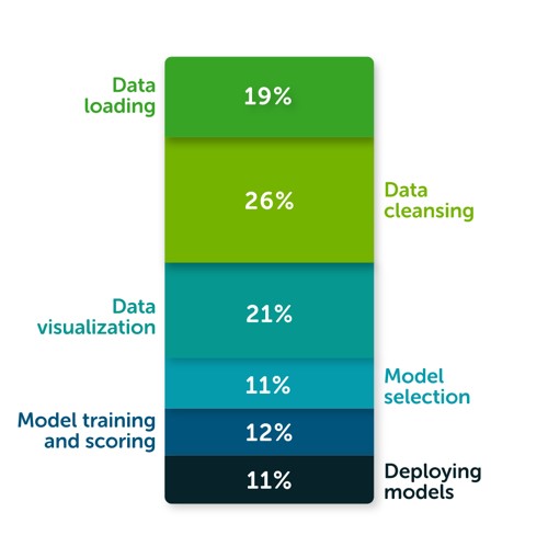
According to The State of Data Science 2020 survey, data management, exploratory data analysis (EDA), feature selection, and feature engineering accounts for more than 66% of a data scientist’s time (see the following diagram).

The same survey highlights that the top three biggest roadblocks to deploying a model in production are managing dependencies and environments, security, and skill gaps (see the following diagram).

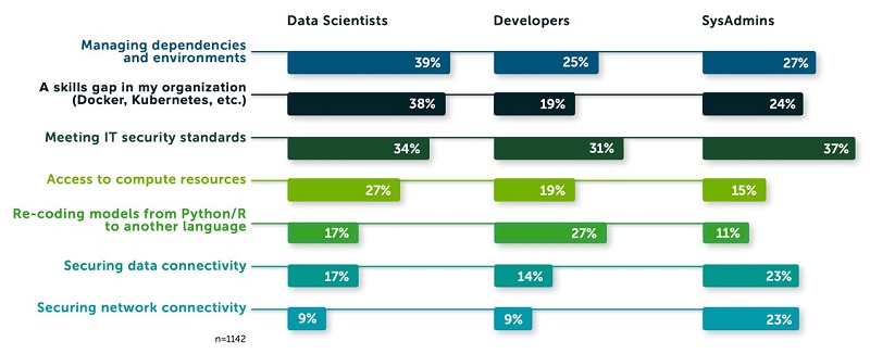
The survey posits that these struggles result in fewer than half (48%) of the respondents feeling able to illustrate the impact data science has on business outcomes.

Enter Amazon SageMaker Data Wrangler, the fastest and easiest way to prepare data for machine learning (ML). SageMaker Data Wrangler gives you the ability to use a visual interface to access data, perform EDA and feature engineering, and seamlessly operationalize your data flow by exporting it into an Amazon SageMaker pipeline, Amazon SageMaker Data Wrangler job, Python file, or SageMaker feature group.

SageMaker Data Wrangler also provides you with over 300 built-in transforms, custom transforms using a Python, PySpark or SparkSQL runtime, built-in data analysis such as common charts (like scatterplot or histogram), custom charts using the Altair library, and useful model analysis capabilities such as feature importance, target leakage, and model explainability. Finally, SageMaker Data Wrangler creates a data flow file that can be versioned and shared across your teams for reproducibility.

Solution overview

In this post, we use the retail demo store example and generate a sample dataset. We use three files: users.csv, items.csv, and interactions.csv. We first prepare the data in order to predict the customer segment based on past interactions. Our target is the field called persona, which we later transform and rename to USER_SEGMENT.

The following code is a preview of the users dataset:

id,username,email,first_name,last_name,addresses,age,gender,persona
1,user1,nathan.smith@example.com,Nathan,Smith,"[{""first_name"": ""Nathan"", ""last_name"": ""Smith"", ""address1"": ""049 Isaac Stravenue Apt. 770"", ""address2"": """", ""country"": ""US"", ""city"": ""Johnsonmouth"", ""state"": ""NY"", ""zipcode"": ""12758"", ""default"": true}]",28,M,electronics_beauty_outdoors
2,user2,kevin.martinez@example.com,Kevin,Martinez,"[{""first_name"": ""Kevin"", ""last_name"": ""Martinez"", ""address1"": ""074 Jennifer Flats Suite 538"", ""address2"": """", ""country"": ""US"", ""city"": ""East Christineview"", ""state"": ""MI"", ""zipcode"": ""49758"", ""default"": true}]",19,M,electronics_beauty_outdoors

The following code is a preview of the items dataset:

ITEM_ID,ITEM_URL,ITEM_SK,ITEM_NAME,ITEM_CATEGORY,ITEM_STYLE,ITEM_DESCRIPTION,ITEM_PRICE,ITEM_IMAGE,ITEM_FEATURED,ITEM_GENDER_AFFINITY
36,http://dbq4nocqaarhp.cloudfront.net/#/product/36,,Exercise Headphones,electronics,headphones,These stylishly red ear buds wrap securely around your ears making them perfect when exercising or on the go.,19.99,5.jpg,true,
49,http://dbq4nocqaarhp.cloudfront.net/#/product/49,,Light Brown Leather Lace-Up Boot,footwear,boot,Sturdy enough for the outdoors yet stylish to wear out on the town.,89.95,11.jpg,,

The following code is a preview of the interactions dataset:

ITEM_ID,USER_ID,EVENT_TYPE,TIMESTAMP
2,2539,ProductViewed,1589580300
29,5575,ProductViewed,1589580305
4,1964,ProductViewed,1589580309
46,5291,ProductViewed,1589580309

This post is not intended to be a step-by-step guide, but rather describe the process of preparing a training dataset and highlight some of the transforms and data analysis capabilities using SageMaker Data Wrangler. You can download the .flow files if you want to download, upload, and retrace the full example in your SageMaker Studio environment.

At a high level, we perform the following steps: 

1. Connect to Amazon Simple Storage Service (Amazon S3) and import the data.
2. Transform the data, including type casting, dropping unneeded columns, imputing missing values, label encoding, one hot encoding, and custom transformations to extract elements from a JSON formatted column.
3. Create table summaries and charts for data analysis. We use the quick model option to get a sense of which features are adding predictive power as we progress with our data preparation. We also use the built-in target leakage capability and get a report on any features that are at risk of leaking.
4. Create a data flow, in which we combine and join the three tables to perform further aggregations and data analysis.
5. Iterate by performing additional feature engineering or data analysis on the newly added data.
6. Export our workflow to a SageMaker Data Wrangler job.

Prerequisites

Make sure you don’t have any quota limits on the m5.4xlarge instance type part of your Studio application before creating a new data flow. For more information about prerequisites, see Getting Started with Data Wrangler.

Importing the data

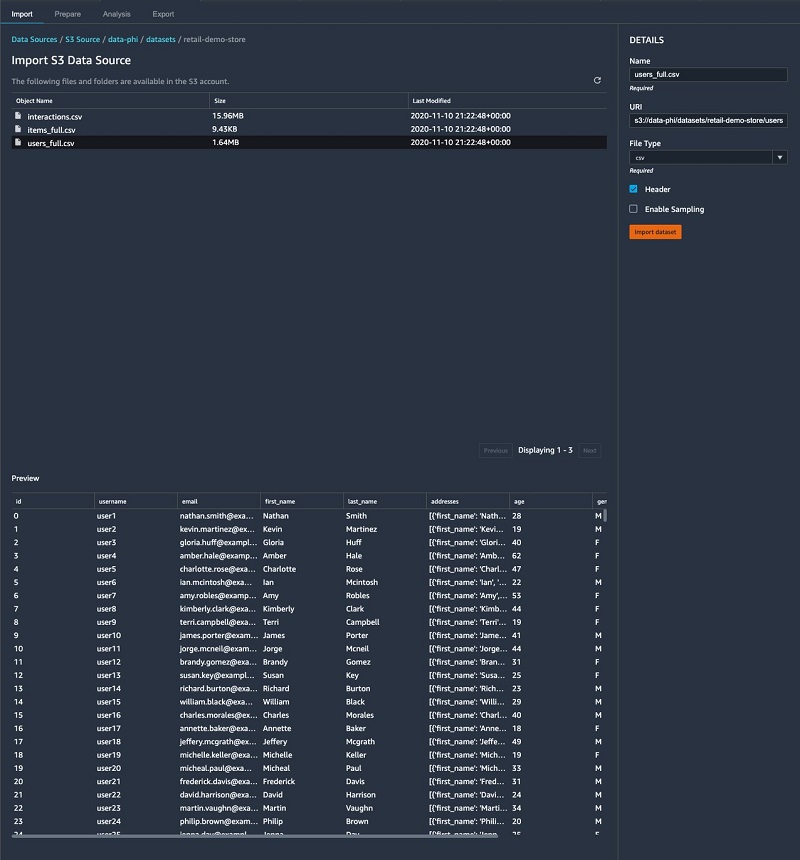
We import our three CSV files from Amazon S3. SageMaker Data Wrangler supports CSV and Parquet files. It also allows you to sample the data in case the data is too large to fit in your studio application. The following screenshot shows a preview of the users dataset.

After importing our CSV files, our datasets look like the following screenshot in SageMaker Data Wrangler.

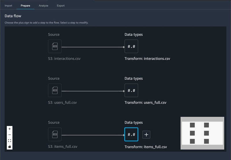
We can now add some transforms and perform data analysis.

Transforming the data

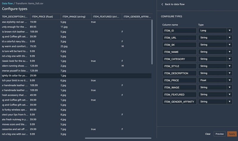
For each table, we check the data types and make sure that it was inferred correctly.

Items table

To perform transforms on the items table, complete the following steps:

1. On the SageMaker Data Wrangler UI, for the items table, choose +.
2. Choose Edit data types.

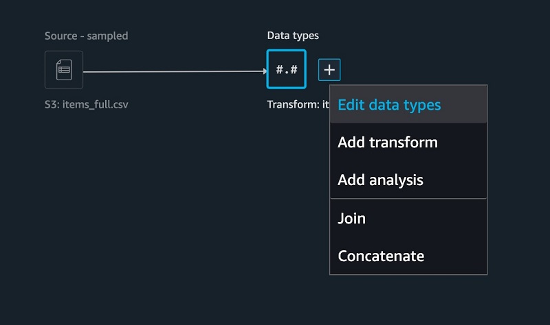
Most of the columns were inferred properly, except for one. The ITEM_FEATURED column is missing values and should really be casted as a Boolean.

For the items table, we perform the following transformations:

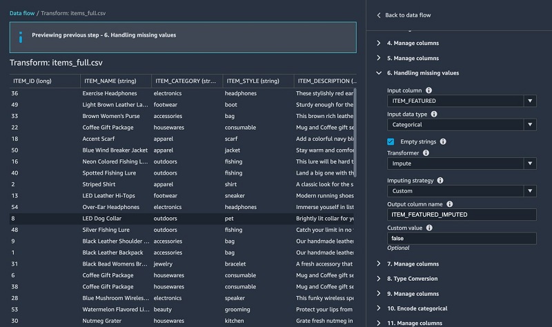
• Fill missing values with false for the ITEM_FEATURED column
• Drop unneeded columns such as URL, SK, IMAGE, NAME, STYLE, ITEM_FEATURED and DESCRIPTION
• Rename ITEM_FEATURED_IMPUTED to ITEM_FEATURED
• Cast the ITEM_FEATURED column as Boolean
• Encode the ITEM_GENDER_AFFINITY column

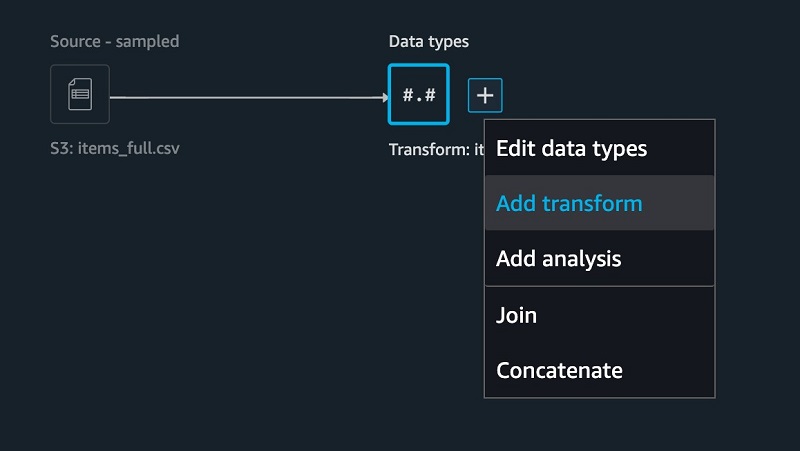
3. To add a new transform, choose + and choose Add transform.

4. Fill in missing values using the built-in Handling missing values transform.

5. To drop columns, under Manage columns, For Input column, choose ITEM_URL.
   1. For Required column operator, choose Drop column.
   2. Repeat this step for SK, IMAGE, NAME, STYLE, ITEM_FEATURED, and DESCRIPTION

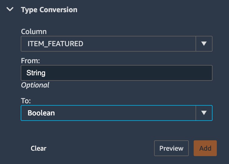
6. Under Type Conversion, for Column, choose ITEM_FEATURED.
7. for To, choose Boolean.

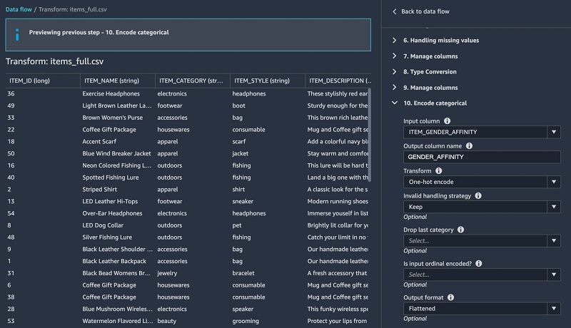
8. Under Encore categorical, add a one hot encoding transform to the ITEM_GENDER_AFFINITY column.

9. Rename our column from ITEM_FEATURED_IMPUTED to ITEM_FEATURED.
10. Run a table summary.

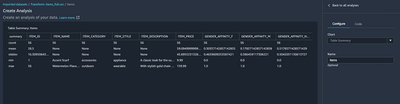
The table summary data analysis doesn’t provide information on all the columns.

11. Run the df.info() function as a custom transform.
12. Choose Preview to verify that our ITEM_FEATURED column comes as a Boolean data type.

DataFrame.info() prints information about the DataFrame including the data types, non-null values, and memory usage.

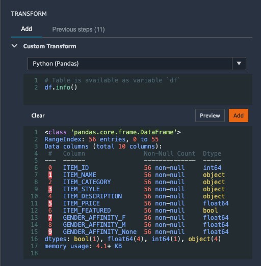
13. Check that the ITEM_FEATURED column has been casted properly and doesn’t have any null values.

Let’s move on to the users table and prepare our dataset for training.

Users table

For the users table, we perform the following steps:

1. Drop unneeded columns such as username, email, first_name, and last_name.
2. Extract elements from a JSON column such as zip code, state, and city.

The addresse column containing a JSON string looks like the following code:

[{  "first_name": "Nathan",
    "last_name": "Smith", 
    "address1": "049 Isaac Stravenue Apt. 770", 
    "address2": "", 
    "country": "US", 
    "city": "Johnsonmouth", 
    "state": "NY", 
    "zipcode": "12758", 
    "default": true
    }]

To extract relevant location elements for our model, we apply several transforms and save them in their respective columns. The following screenshot shows an example of extracting the user zip code.

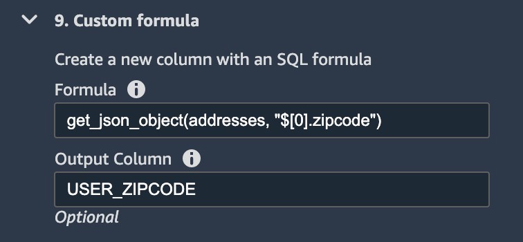
We apply the same transform to extract city and state, respectively.

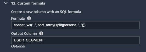
3. In the following transform, we split and rearrange the different personas (such as electronics_beauty_outdoors) and save it as USER_SEGMENT.

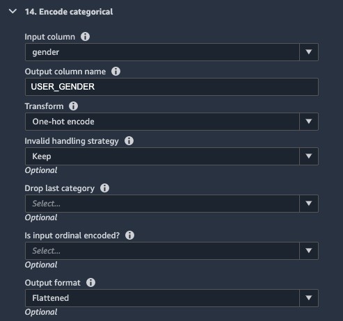
4. We also perform a one hot encoding on the USER_GENDER column.

Interactions table

Finally, in the interactions table, we complete the following steps:

1. Perform a custom transform to extract the event date and time from a timestamp.

Custom transforms are quite powerful because they allow you to insert a snippet of code and run the transform using different runtime engines such as PySpark, Python, or SparkSQL. All you have to do is to start your transform with df, which denotes the DataFrame.

The following code is an example using a custom PySpark transform to extract the date and time from the timestamp:

from pyspark.sql.functions import from_unixtime, to_date, date_format
df = df.withColumn('DATE_TIME', from_unixtime('TIMESTAMP'))
df = df.withColumn(  'EVENT_DATE', to_date('DATE_TIME')).withColumn(  'EVENT_TIME', date_format('DATE_TIME', 'HH:mm:ss'))

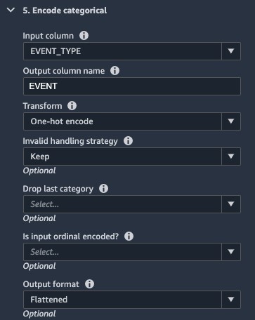
2. Perform a one hot encoding on the EVENT_TYPE

3. Lastly, drop any columns we don’t need.

Performing data analysis

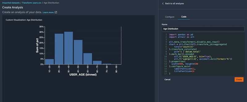
In addition to common built-in data analysis such as scatterplots and histograms, SageMaker Data Wrangler gives you the ability to build custom visualizations using the Altair library.

In the following histogram chart, we binned the user by age ranges on the x axis and the total percentage of users on the y axis.

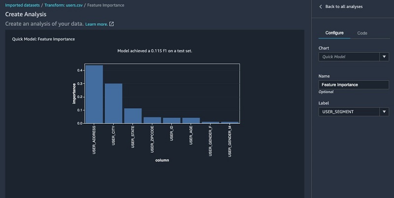
We can also use the quick model functionality to show feature importance. The F1 score indicating the model’s predictive accuracy is also shown in the following visualization. This enables you to iterate by adding new datasets and performing additional features engineering to incrementally improve model accuracy.

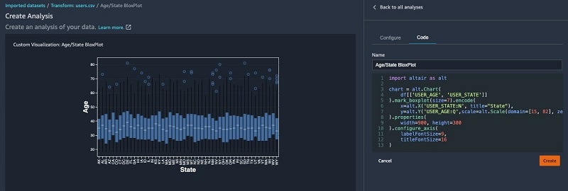
The following visualization is a box plot by age and state. This is particularly useful to understand the interquartile range and possible outliers.

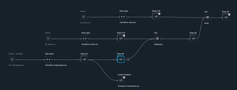
Building a data flow

SageMaker Data Wrangler builds a data flow and keeps the dependencies of all the transforms, data analysis, and table joins. This allows you to keep a lineage of your exploratory data analysis but also allows you to reproduce past experiments consistently.

In this section, we join our interactions and items tables.

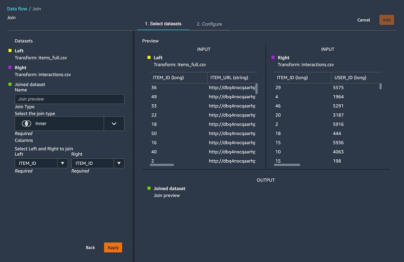
1. Join our tables using the ITEM_ID key.
2. Use a custom transform to aggregate our dataset by USER_ID and generate other features by pivoting the ITEM_CATEGORY and EVENT_TYPE:

import pyspark.sql.functions as F
df = df.groupBy(["USER_ID"]).pivot("ITEM_CATEGORY")
.agg(F.sum("EVENT_TYPE_PRODUCTVIEWED").alias("EVENT_TYPE_PRODUCTVIEWED"),	
F.sum("EVENT_TYPE_PRODUCTADDED").alias("EVENT_TYPE_PRODUCTADDED"),	
F.sum("EVENT_TYPE_CARTVIEWED").alias("EVENT_TYPE_CARTVIEWED"),	
F.sum("EVENT_TYPE_CHECKOUTSTARTED").alias("EVENT_TYPE_CHECKOUTSTARTED"),	
F.sum("EVENT_TYPE_ORDERCOMPLETED").alias("EVENT_TYPE_ORDERCOMPLETED"),	
F.sum(F.col("ITEM_PRICE") * F.col("EVENT_TYPE_ORDERCOMPLETED")).alias("TOTAL_REVENUE"),	
F.avg(F.col("ITEM_FEATURED").cast("integer")).alias("FEATURED_ITEM_FRAC"),	
F.avg("GENDER_AFFINITY_F").alias("FEM_AFFINITY_FRAC"),	
F.avg("GENDER_AFFINITY_M").alias("MASC_AFFINITY_FRAC")).fillna(0)

3. Join our dataset with the users tables.

The following screenshot shows what our DAG looks like after joining all the tables together.

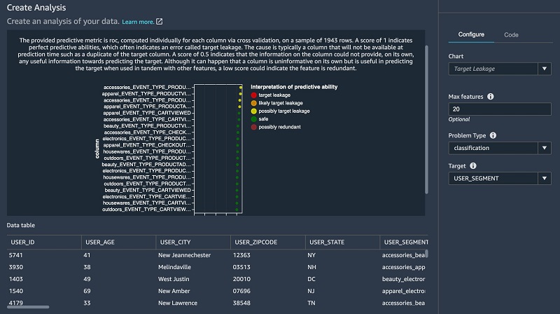
4. Now that we have combined all three tables, run data analysis for target leakage.

Target leakage or data leakage is one of the most common and difficult problems when building a model. Target leakages mean that you use features as part of training your model that aren’t available upon inference time. For example, if you try to predict a car crash and one of the features is airbag_deployed, you don’t know if the airbag has been deployed until the crash happened.

The following screenshot shows that we don’t have a strong target leakage candidate after running the data analysis.

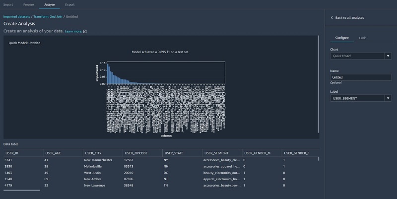
5. Finally, we run a quick model on the joined dataset.

The following screenshot shows that our F1 score is 0.89 after joining additional data and performing further feature transformations.

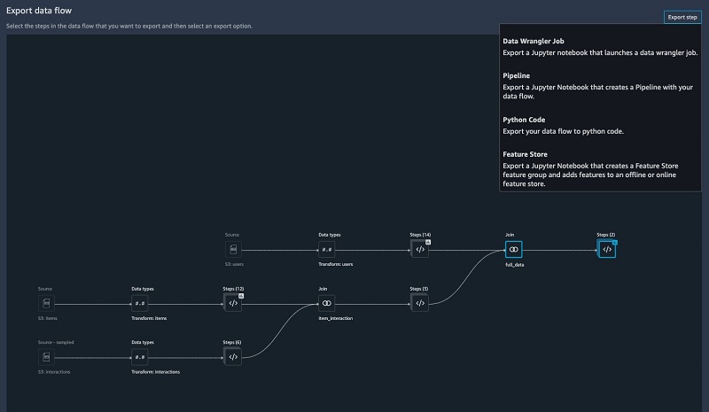
Exporting your data flow

SageMaker Data Wrangler gives you the ability to export your data flow into a Jupyter notebook with code pre-populated for the following options:

• SageMaker Data Wrangler job
• SageMaker Pipelines
• SageMaker Feature Store

SageMaker Data Wrangler can also output a Python file.

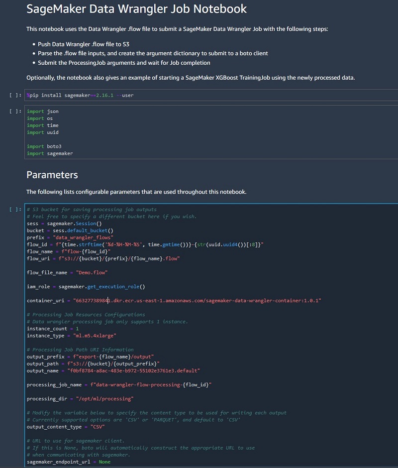
The SageMaker Data Wrangler job pre-populated in a Jupyter notebook ready to be run.

Conclusion

SageMaker Data Wrangler makes it easy to ingest data and perform data preparation tasks such as exploratory data analysis, feature selection, feature engineering, and more advanced data analysis such as feature importance, target leakage, and model explainability using an easy and intuitive user interface. SageMaker Data Wrangler makes the transition of converting your data flow into an operational artifact such as a SageMaker Data Wrangler job, SageMaker feature store, or SageMaker pipeline very easy with one click of a button.

Log in into your Studio environment, download the .flow file, and try SageMaker Data Wrangler today.

About the Authors

Phi Nguyen is a solution architect at AWS helping customers with their cloud journey with a special focus on data lake, analytics, semantics technologies and machine learning. In his spare time, you can find him biking to work, coaching his son’s soccer team or enjoying nature walk with his family.

Roberto Bruno Martins is a Machine Learning Specialist Solution Architect, helping customers from several industries create, deploy and run machine learning solutions. He’s been working with data since 1994, and has no plans to stop any time soon. In his spare time he plays games, practices martial arts and likes to try new food.