Apache MXNet Version 0.12 Extends Gluon Functionality to Support Cutting Edge Research

Last week, the Apache MXNet community released version 0.12 of MXNet. The major features were support for NVIDIA Volta GPUs and sparse tensors. The release also included a number of new features for the Gluon programming interface. In particular, these features make it easier to implement cutting-edge research in your deep learning models:

• Variational dropout, which enables you to effectively apply the dropout technique for mitigating overfitting to recurrent neural networks (RNNs)
• Convolutional RNN, Long short-term memory (LSTM), and gated recurrent unit (GRU) Cells, which allow modeling of datasets exhibiting both time-based sequence and spatial dimensions
• Seven new loss functions, export functionality, and trainer function enhancements

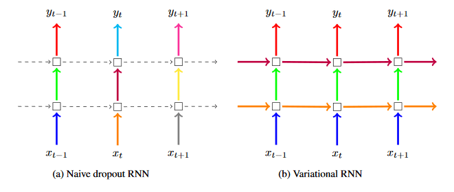
Variational dropout (VariationalDropoutCell) builds on recent research to provide a new tool for mitigating overfitting in RNNs. It draws from “A Theoretically Grounded Application of Recurrent Neural Networks” and “RNNDrop: A Novel Approach for RNNs in ASR.” Overfitting is a modeling error where the model is fit so closely to the training dataset that it diminishes its prediction accuracy when it sees new data or the test dataset. Dropout is a modeling technique that randomly zeroes out model parameters, so that the model doesn’t become overly dependent on any single input or parameter during training. However, this technique hasn’t been applied successfully to RNNs. Research to date has focused on applying dropout only to the inputs and outputs with complete randomness in what is zeroed out across all of the RNN’s time steps. Variational Dropout eliminates this randomness across time steps and applies the same random dropout array (or mask) to the RNN’s inputs, outputs, and hidden states at each time step.

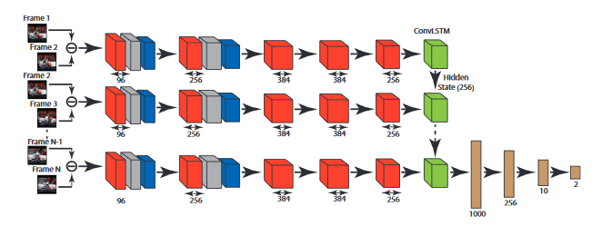
The convolutional RNN, LSTM, and GRU cells (e.g., Conv1DRNNCell, Conv1DLSTMCell, Conv1DGRUCell) make it easier to model datasets that have both sequence and spatial dimensions – for example, videos or images captured over time. Convolutional LSTM models were first successfully applied in research presented in “Convolutional LSTM Network: A Machine Learning Approach for Precipitation Nowcasting.” LSTM networks are designed for analyzing sequential data while keeping track of long-term dependencies. They have advanced the state of the art in natural language processing (NLP). However, they perform with limited effectiveness when applied to spatiotemporal use cases where the dataset has a spatial dimension in addition to exhibiting a time-based sequence. Examples of spatiotemporal use cases include predicting total volume of rainfall in different pockets of Hong Kong in the next six hours (as discussed in the research paper referenced earlier) or detecting whether a video is violent. For image recognition, convolutional neural networks (CNNs) advanced the state of the art by applying a convolution operation on images, enabling the model to capture spatial context. Convolutional RNN, LSTMs, and GRUs incorporate these convolution operations into the RNN, LSTM, and GRU architectures, respectively.

This MXNet release also expanded the set of supported loss functions in Gluon by seven: (1) sigmoid binary cross entropy loss, (2) connectionist temporal classification (CTC) loss, (3) Huber loss, (4) hinge loss, (5) squared hinge loss, (6) logistic loss, and (7) triple loss. Loss functions measure how well your model is performing according to some objective. These loss functions use different mathematical computations to measure this performance, and thus they have different effects on the optimization process during model training. Choosing a loss function is more of an art than a science, and there is no simple heuristic for deciding which one to select. Instead, you can examine the extensive research on each these loss functions to get a perspective on when these loss functions were applied successfully and when not so successfully.

This release also introduces helpful additions like an export API and a learning rate property for the trainer optimizer function. The export API enables you to export your neural network model architecture and the associated model parameters to an intermediary format that can used to load the model at a later point or in a different location. This API is still experimental, so all functionality isn’t yet supported. In addition, you can now set and read the learning rate using the newly added learning rate property of trainer.

Next steps

Getting started with MXNet is simple, and a full list of changes in this release can be found in the release notes. To learn more about the Gluon interface, visit the MXNet details page.

About the Author

Vikram Madan is a Senior Product Manager for AWS Deep Learning. He works on products that make deep learning engines easier to use with a specific focus on the open source Apache MXNet engine. In his spare time, he enjoys running long distances and watching documentaries.