Analyze OpenFDA Data in R with Amazon S3 and Amazon Athena

One of the great benefits of Amazon S3 is the ability to host, share, or consume public data sets. This provides transparency into data to which an external data scientist or developer might not normally have access. By exposing the data to the public, you can glean many insights that would have been difficult with a data silo.

The openFDA project creates easy access to the high value, high priority, and public access data of the Food and Drug Administration (FDA). The data has been formatted and documented in consumer-friendly standards. Critical data related to drugs, devices, and food has been harmonized and can easily be called by application developers and researchers via API calls. In addition, FDA makes openFDA data available on S3 in raw format.

In this post, I show how to use S3, Amazon EMR, and Amazon Athena to analyze the drug adverse events dataset. A drug adverse event is an undesirable experience associated with the use of a drug, including serious drug side effects, product use errors, product quality programs, and therapeutic failures.

Data considerations

Keep in mind that this data does have limitations. In addition, in the United States, these adverse events are submitted to the FDA voluntarily from consumers so there may not be reports for all events that occurred. There is no certainty that the reported event was actually due to the product. The FDA does not require that a causal relationship between a product and event be proven, and reports do not always contain the detail necessary to evaluate an event. Because of this, there is no way to identify the true number of events. The important takeaway to all this is that the information contained in this data has not been verified to produce cause and effect relationships. Despite this disclaimer, many interesting insights and value can be derived from the data to accelerate drug safety research.

Data analysis using SQL

For application developers who want to perform targeted searching and lookups, the API endpoints provided by the openFDA project are “ready to go” for software integration using a standard API powered by Elasticsearch, NodeJS, and Docker. However, for data analysis purposes, it is often easier to work with the data using SQL and statistical packages that expect a SQL table structure. For large-scale analysis, APIs often have query limits, such as 5000 records per query. This can cause extra work for data scientists who want to analyze the full dataset instead of small subsets of data.

To address the concern of requiring all the data in a single dataset, the openFDA project released the full 100 GB of harmonized data files that back the openFDA project onto S3. Athena is an interactive query service that makes it easy to analyze data in S3 using standard SQL. It’s a quick and easy way to answer your questions about adverse events and aspirin that does not require you to spin up databases or servers.

While you could point tools directly at the openFDA S3 files, you can find greatly improved performance and use of the data by following some of the preparation steps later in this post.

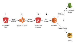
Architecture

This post explains how to use the following architecture to take the raw data provided by openFDA, leverage several AWS services, and derive meaning from the underlying data.

Steps:

Load the openFDA /drug/event dataset into Spark and convert it to gzip to allow for streaming.
Transform the data in Spark and save the results as a Parquet file in S3.
Query the S3 Parquet file with Athena.
Perform visualization and analysis of the data in R and Python on Amazon EC2.

Optimizing public data sets: A primer on data preparation

Those who want to jump right into preparing the files for Athena may want to skip ahead to the next section.

Transforming, or pre-processing, files is a common task for using many public data sets. Before you jump into the specific steps for transforming the openFDA data files into a format optimized for Athena, I thought it would be worthwhile to provide a quick exploration on the problem.

Making a dataset in S3 efficiently accessible with minimal transformation for the end user has two key elements:

Partitioning the data into objects that contain a complete part of the data (such as data created within a specific month).
Using file formats that make it easy for applications to locate subsets of data (for example, gzip, Parquet, ORC, etc.).

With these two key elements in mind, you can now apply transformations to the openFDA adverse event data to prepare it for Athena. You might find the data techniques employed in this post to be applicable to many of the questions you might want to ask of the public data sets stored in Amazon S3.

Before you get started, I encourage those who are interested in doing deeper healthcare analysis on AWS to make sure that you first read the AWS HIPAA Compliance whitepaper. This covers the information necessary for processing and storing protected health information (PHI).

Also, the adverse event analysis shown for aspirin is strictly for demonstration purposes and should not be used for any real decision or taken as anything other than a demonstration of AWS capabilities. However, there have been robust case studies published that have explored a causal relationship between aspirin and adverse reactions using OpenFDA data. If you are seeking research on aspirin or its risks, visit organizations such as the Centers for Disease Control and Prevention (CDC) or the Institute of Medicine (IOM).

Preparing data for Athena

For this walkthrough, you will start with the FDA adverse events dataset, which is stored as JSON files within zip archives on S3. You then convert it to Parquet for analysis. Why do you need to convert it? The original data download is stored in objects that are partitioned by quarter.

Here is a small sample of what you find in the adverse events (/drugs/event) section of the openFDA website.

If you were looking for events that happened in a specific quarter, this is not a bad solution. For most other scenarios, such as looking across the full history of aspirin events, it requires you to access a lot of data that you won’t need. The zip file format is not ideal for using data in place because zip readers must have random access to the file, which means the data can’t be streamed. Additionally, the zip files contain large JSON objects.

To read the data in these JSON files, a streaming JSON decoder must be used or a computer with a significant amount of RAM must decode the JSON. Opening up these files for public consumption is a great start. However, you still prepare the data with a few lines of Spark code so that the JSON can be streamed.

Step 1: Convert the file types

Using Apache Spark on EMR, you can extract all of the zip files and pull out the events from the JSON files. To do this, use the Scala code below to deflate the zip file and create a text file. In addition, compress the JSON files with gzip to improve Spark’s performance and reduce your overall storage footprint. The Scala code can be run in either the Spark Shell or in an Apache Zeppelin notebook on your EMR cluster.

If you are unfamiliar with either Apache Zeppelin or the Spark Shell, the following posts serve as great references:

import scala.io.Source
import java.util.zip.ZipInputStream
import org.apache.spark.input.PortableDataStream
import org.apache.hadoop.io.compress.GzipCodec

// Input Directory
val inputFile = "s3://download.open.fda.gov/drug/event/2015q4/*.json.zip";

// Output Directory
val outputDir = "s3://{YOUR OUTPUT BUCKET HERE}/output/2015q4/";

// Extract zip files from 
val zipFiles = sc.binaryFiles(inputFile);

// Process zip file to extract the json as text file and save it
// in the output directory 
val rdd = zipFiles.flatMap((file: (String, PortableDataStream)) => {
    val zipStream = new ZipInputStream(file.2.open)
    val entry = zipStream.getNextEntry
    val iter = Source.fromInputStream(zipStream).getLines
    iter
}).map(.replaceAll("\s+","")).saveAsTextFile(outputDir, classOf[GzipCodec])

Step 2: Transform JSON into Parquet

With just a few more lines of Scala code, you can use Spark’s abstractions to convert the JSON into a Spark DataFrame and then export the data back to S3 in Parquet format.

Spark requires the JSON to be in JSON Lines format to be parsed correctly into a DataFrame.

// Output Parquet directory
val outputDir = "s3://{YOUR OUTPUT BUCKET NAME}/output/drugevents"
// Input json file
val inputJson = "s3://{YOUR OUTPUT BUCKET NAME}/output/2015q4/*"
// Load dataframe from json file multiline 
val df = spark.read.json(sc.wholeTextFiles(inputJson).values)
// Extract results from dataframe
val results = df.select("results")
// Save it to Parquet
results.write.parquet(outputDir)

Step 3: Create an Athena table

With the data cleanly prepared and stored in S3 using the Parquet format, you can now place an Athena table on top of it to get a better understanding of the underlying data.

Because the openFDA data structure incorporates several layers of nesting, it can be a complex process to try to manually derive the underlying schema in a Hive-compatible format. To shorten this process, you can load the top row of the DataFrame from the previous step into a Hive table within Zeppelin and then extract the “create table” statement from SparkSQL.

results.createOrReplaceTempView("data")

val top1 = spark.sql("select * from data tablesample(1 rows)")

top1.write.format("parquet").mode("overwrite").saveAsTable("drugevents")

val show_cmd = spark.sql("show create table drugevents”).show(1, false)

This returns a “create table” statement that you can almost paste directly into the Athena console. Make some small modifications (adding the word “external” and replacing “using with “stored as”), and then execute the code in the Athena query editor. The table is created.

For the openFDA data, the DDL returns all string fields, as the date format used in your dataset does not conform to the yyy-mm-dd hh:mm:ss[.f…] format required by Hive. For your analysis, the string format works appropriately but it would be possible to extend this code to use a Presto function to convert the strings into time stamps.

CREATE EXTERNAL TABLE  drugevents (
   companynumb  string, 
   safetyreportid  string, 
   safetyreportversion  string, 
   receiptdate  string, 
   patientagegroup  string, 
   patientdeathdate  string, 
   patientsex  string, 
   patientweight  string, 
   serious  string, 
   seriousnesscongenitalanomali  string, 
   seriousnessdeath  string, 
   seriousnessdisabling  string, 
   seriousnesshospitalization  string, 
   seriousnesslifethreatening  string, 
   seriousnessother  string, 
   actiondrug  string, 
   activesubstancename  string, 
   drugadditional  string, 
   drugadministrationroute  string, 
   drugcharacterization  string, 
   drugindication  string, 
   drugauthorizationnumb  string, 
   medicinalproduct  string, 
   drugdosageform  string, 
   drugdosagetext  string, 
   reactionoutcome  string, 
   reactionmeddrapt  string, 
   reactionmeddraversionpt  string)
STORED AS parquet
LOCATION
  's3://{YOUR TARGET BUCKET}/output/drugevents'

With the Athena table in place, you can start to explore the data by running ad hoc queries within Athena or doing more advanced statistical analysis in R.

Using SQL and R to analyze adverse events

Using the openFDA data with Athena makes it very easy to translate your questions into SQL code and perform quick analysis on the data. After you have prepared the data for Athena, you can begin to explore the relationship between aspirin and adverse drug events, as an example. One of the most common metrics to measure adverse drug events is the Proportional Reporting Ratio (PRR). It is defined as:

PRR = (m/n)/( (M-m)/(N-n) )
Where
m = #reports with drug and event
n = #reports with drug
M = #reports with event in database
N = #reports in database

Gastrointestinal haemorrhage has the highest PRR of any reaction to aspirin when viewed in aggregate. One question you may want to ask is how the PRR has trended on a yearly basis for gastrointestinal haemorrhage since 2005.

Using the following query in Athena, you can see the PRR trend of “GASTROINTESTINAL HAEMORRHAGE” reactions with “ASPIRIN” since 2005:

with drug_and_event as 
(select rpad(receiptdate, 4, 'NA') as receipt_year
    , reactionmeddrapt
    , count(distinct (concat(safetyreportid,receiptdate,reactionmeddrapt))) as reports_with_drug_and_event 
from fda.drugevents
where rpad(receiptdate,4,'NA') 
     between '2005' and '2015' 
     and medicinalproduct = 'ASPIRIN'
     and reactionmeddrapt= 'GASTROINTESTINAL HAEMORRHAGE'
group by reactionmeddrapt, rpad(receiptdate, 4, 'NA') 
), reports_with_drug as 
(
select rpad(receiptdate, 4, 'NA') as receipt_year
    , count(distinct (concat(safetyreportid,receiptdate,reactionmeddrapt))) as reports_with_drug 
 from fda.drugevents 
 where rpad(receiptdate,4,'NA') 
     between '2005' and '2015' 
     and medicinalproduct = 'ASPIRIN'
group by rpad(receiptdate, 4, 'NA') 
), reports_with_event as 
(
   select rpad(receiptdate, 4, 'NA') as receipt_year
    , count(distinct (concat(safetyreportid,receiptdate,reactionmeddrapt))) as reports_with_event 
   from fda.drugevents
   where rpad(receiptdate,4,'NA') 
     between '2005' and '2015' 
     and reactionmeddrapt= 'GASTROINTESTINAL HAEMORRHAGE'
   group by rpad(receiptdate, 4, 'NA')
), total_reports as 
(
   select rpad(receiptdate, 4, 'NA') as receipt_year
    , count(distinct (concat(safetyreportid,receiptdate,reactionmeddrapt))) as total_reports 
   from fda.drugevents
   where rpad(receiptdate,4,'NA') 
     between '2005' and '2015' 
   group by rpad(receiptdate, 4, 'NA')
)
select  drug_and_event.receipt_year, 
(1.0 * drug_and_event.reports_with_drug_and_event/reports_with_drug.reports_with_drug)/ (1.0 * (reports_with_event.reports_with_event- drug_and_event.reports_with_drug_and_event)/(total_reports.total_reports-reports_with_drug.reports_with_drug)) as prr
, drug_and_event.reports_with_drug_and_event
, reports_with_drug.reports_with_drug
, reports_with_event.reports_with_event
, total_reports.total_reports
from drug_and_event
    inner join reports_with_drug on  drug_and_event.receipt_year = reports_with_drug.receipt_year   
    inner join reports_with_event on  drug_and_event.receipt_year = reports_with_event.receipt_year
    inner join total_reports on  drug_and_event.receipt_year = total_reports.receipt_year
order by  drug_and_event.receipt_year

One nice feature of Athena is that you can quickly connect to it via R or any other tool that can use a JDBC driver to visualize the data and understand it more clearly.

With this quick R script that can be run in R Studio either locally or on an EC2 instance, you can create a visualization of the PRR and Reporting Odds Ratio (RoR) for “GASTROINTESTINAL HAEMORRHAGE” reactions from “ASPIRIN” since 2005 to better understand these trends.

# connect to ATHENA
conn <- dbConnect(drv, '<Your JDBC URL>',s3_staging_dir="<Your S3 Location>",user=Sys.getenv(c("USER_NAME"),password=Sys.getenv(c("USER_PASSWORD"))

# Declare Adverse Event
adverseEvent <- "'GASTROINTESTINAL HAEMORRHAGE'"

# Build SQL Blocks
sqlFirst <- "SELECT rpad(receiptdate, 4, 'NA') as receipt_year, count(DISTINCT safetyreportid) as event_count FROM fda.drugsflat WHERE rpad(receiptdate,4,'NA') between '2005' and '2015'"
sqlEnd <- "GROUP BY rpad(receiptdate, 4, 'NA') ORDER BY receipt_year"

# Extract Aspirin with adverse event counts
sql <- paste(sqlFirst,"AND medicinalproduct ='ASPIRIN' AND reactionmeddrapt=",adverseEvent, sqlEnd,sep=" ")
aspirinAdverseCount = dbGetQuery(conn,sql)

# Extract Aspirin counts
sql <- paste(sqlFirst,"AND medicinalproduct ='ASPIRIN'", sqlEnd,sep=" ")
aspirinCount = dbGetQuery(conn,sql)

# Extract adverse event counts
sql <- paste(sqlFirst,"AND reactionmeddrapt=",adverseEvent, sqlEnd,sep=" ")
adverseCount = dbGetQuery(conn,sql)

# All Drug Adverse event Counts
sql <- paste(sqlFirst, sqlEnd,sep=" ")
allDrugCount = dbGetQuery(conn,sql)

# Select correct rows
selAll =  allDrugCount$receipt_year == aspirinAdverseCount$receipt_year
selAspirin = aspirinCount$receipt_year == aspirinAdverseCount$receipt_year
selAdverse = adverseCount$receipt_year == aspirinAdverseCount$receipt_year

# Calculate Numbers
m <- c(aspirinAdverseCount$event_count)
n <- c(aspirinCount[selAspirin,2])
M <- c(adverseCount[selAdverse,2])
N <- c(allDrugCount[selAll,2])

# Calculate proptional reporting ratio
PRR = (m/n)/((M-m)/(N-n))

# Calculate reporting Odds Ratio
d = n-m
D = N-M
ROR = (m/d)/(M/D)

# Plot the PRR and ROR
g_range <- range(0, PRR,ROR)
g_range[2] <- g_range[2] + 3
yearLen = length(aspirinAdverseCount$receipt_year)
axis(1,1:yearLen,lab=ax)
plot(PRR, type="o", col="blue", ylim=g_range,axes=FALSE, ann=FALSE)
axis(1,1:yearLen,lab=ax)
axis(2, las=1, at=1*0:g_range[2])
box()
lines(ROR, type="o", pch=22, lty=2, col="red")

As you can see, the PRR and RoR have both remained fairly steady over this time range. With the R Script above, all you need to do is change the adverseEvent variable from GASTROINTESTINAL HAEMORRHAGE to another type of reaction to analyze and compare those trends.

Summary

In this walkthrough:

You used a Scala script on EMR to convert the openFDA zip files to gzip.
You then transformed the JSON blobs into flattened Parquet files using Spark on EMR.
You created an Athena DDL so that you could query these Parquet files residing in S3.
Finally, you pointed the R package at the Athena table to analyze the data without pulling it into a database or creating your own servers.

If you have questions or suggestions, please comment below.

Next Steps

Take your skills to the next level. Learn how to optimize Amazon S3 for an architecture commonly used to enable genomic data analysis. Also, be sure to read more about running R on Amazon Athena.

About the Authors

Ryan Hood is a Data Engineer for AWS. He works on big data projects leveraging the newest AWS offerings. In his spare time, he enjoys watching the Cubs win the World Series and attempting to Sous-vide anything he can find in his refrigerator.

Vikram Anand is a Data Engineer for AWS. He works on big data projects leveraging the newest AWS offerings. In his spare time, he enjoys playing soccer and watching the NFL & European Soccer leagues.

Dave Rocamora is a Solutions Architect at Amazon Web Services on the Open Data team. Dave is based in Seattle and when he is not opening data, he enjoys biking and drinking coffee outside.

AWS Big Data Blog