Using a digital twin for sensitivity analysis to determine sensor placement in a roll-to-roll manufacturing web-line

This post was contributed by Ross Pivovar, Solution Architect, and Adam Rasheed, Head of Emerging Workloads & Technologies, AWS and Orang Vahid, Director of Engineering Services and Kayla Rossi, Application Engineer, Maplesoft

In our previous posts we discussed how to setup a Level 4 Digital Twin (DT) that adapts to changing environments and how to use the L4 DT to perform forecasting, scenario analysis, and risk assessment based on incoming measurement data. In this post today, we’ll discuss methods to find the optimal number, type, and placement of sensors to maximize the accuracy of your Level 3 or Level 4 DT. If you need a refresher, you can check out the AWS digital twin leveling framework. In practice, we don’t have the luxury of adding thousands of sensors to our system. Sensors incur a capital cost, require maintenance and calibration by technicians, inevitably fail (requiring replacement), and they need actual physical space to be installed. In contrast, too few sensors and we miss valuable data that could indicate performance issues, possible system failures, and potential safety issues. For complicated systems or system-of-systems, the number of variables of interest can range from tens to thousands. Hence, it becomes quite difficult and tedious to manually understand the relationship between different factors that impact the performance of the overall system.

In this post, we leverage a combination of our MapleSim DT, machine learning (ML) models, and Shapley sensitivity studies to analyze the relationships between different variables and identify the best sensor placement to trade-off cost versus prediction capability. A sensitivity analysis determines how responsive your engineering models’ outputs are to changes in key input parameters, identifying which variables have the greatest impact on the results. We use TwinFlow to deploy and execute our studies on AWS. We also briefly explore how generative AI can assist in sensor selection.

Where are sensors needed, what type, and how many

As in the prior posts, we consider the web-handling process in roll-to-roll manufacturing for continuous materials like paper, film, and textiles. This example web-handling process involves unwinding the material from a spool, guiding it through various treatments like printing or coating, and then winding it onto individual rolls.

Figure 1 is a schematic diagram of the same roll-to-roll manufacturing line discussed in those earlier posts. The manufacturing line consists of 9 rollers (labeled with “R”) and 12 material spans (labeled with “S”). The operator’s goal is to maximize throughput/yield of the manufacturing line without damaging the product or creating safety hazards. It is critical to monitor various stages in the process for quality control.

It’s tempting to instrument each span or roller with pressure gauges, load cells (to measure tension), feed line sensors (for linear velocity), and roller tachometers (RPM) sensors to track the progress of the roll-to-roll material in the line. This is rarely practical however, due to the high cost of installing and maintaining the sensors. Furthermore, in some cases, there may not be physical space in the facility for all of them.

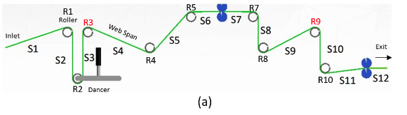
Figure 1 Schematic diagram of the web-handling equipment in which each span is labeled as S1 through S12 and rollers are label R1 through R10.

For our use case, it is known that the minimum information needed to prevent product quality issues include the tension in the material of each span and whether the material is dragging over the rollers (slip) instead of rotating with the rollers.

When considering how to efficiently avoid quality issues, the questions to be answered are:

• When is tension above 175 Newtons (a tension failure threshold)?
• When is slip velocity greater than 1×10^-3 m/s (a differential velocity failure threshold)?
• Which sensors are needed to monitor these failure mechanisms?
• Are all sensor locations needed?
• Can downstream sensors provide information about upstream effects?
• Is there sensor redundancy?

In this example we have at least 42 potential sensors to be included in our manufacturing line. One option is to install sensors to directly measure the tension and differential velocity at all locations. This is not a viable solution for operators due to the cost of installing and maintaining the tension load cells and velocity sensors.

Instead, we can use a digital twin which provides a physics-based simulation of the process, enabling the combination of sensor data with predictions. A digital twin provides both insights into the process and the potential to answer our questions listed above. Our goal changes from directly measuring with physical sensors to identifying which combination of sensors can be used to calibrate a digital twin such that we can create high-accuracy virtual sensors.

Specifically, for our example model of the manufacturing line, the digital twin requires calibration of the roller viscous damping coefficients (see Figure 2). The roller viscous damping coefficient refers to a parameter that can’t be directly measured but reflects the bearing loss due to internal friction as the rollers rotate.  Once the viscous damping coefficients in the model are calibrated, the remaining properties of interest that we want to measure with sensors can instead be predicted purely based on the physics in the model. The question then remains, which sensors do we need in the roll-to-roll manufacturing line to calibrate the viscous damping coefficients in the model?

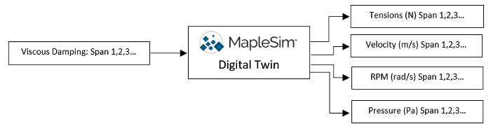
Figure 2 The inputs and outputs of the roll-to-roll manufacturing web line digital twin.

Finding correlations in complicated systems

To determine which sensors are needed to calibrate a model, a traditional approach is to use one-at-a-time perturbations in which a user alters one variable at a time within the model. While simple, this method misses cross-correlation/interactions that are often present within the physical phenomena of the system.

More advanced methods like Sobel sensitivities rely on Monte Carlo sampling to numerically determine both main effects and interactions. Monte Carlo sampling consists of running a simulation model repeatedly (thousands of times), with each simulation using slightly different inputs. The correlation between the inputs and the outputs can then be quantified in a probabilistic manner for further analysis.

However, Sobel sensitivities can potentially provide incorrect results for highly non-linear systems, miss complicated interactions, or are unable to decouple correlated inputs. Additionally, the Sobel sensitivities are designed for global sensitivities.

The method of choice in this blog post, albeit not exclusively better, is to use Shapley sensitivities. Common implementations use an ML model to learn from the Monte Carlo simulations, and then apply game theory to assess the main effects and interactions, regardless of non-linearities or complicated interactions.

Even better, the method can provide sensitivities that either summarize effects across the entire modeling space (global sensitivities) or look at effects locally around a specific point in the space (local sensitivities).

Deploying our MapleSim digital twin on AWS using TwinFlow, we can generate a large sample set (10,000 simulations) to assess the Shapley sensitivities. We can either graphically review the Shapley sensitivities (shown in Figure 3) or look at the raw output (saved to SQL or csv file). For our specific example we have 12 spans and 9 rollers, with 2 properties each resulting in a total of 270 sensitivities relating the viscous damping coefficients (b-labels) to our desired outputs.

Graphically reviewing the sensitivities enables an ad-hoc assessment of the magnitudes. For example, in Figure 3a, we see the sensitivity of the R1 (roller 1) slip velocity to the damping coefficients in each of the rollers. It’s clear that the R1 slip velocity is most sensitive to the damping coefficient of the first roller (labeled b1) and positively correlated (meaning R1 slip velocity increases as the R1 damping coefficient increases).

The damping coefficient for the other rollers (b2 – b10) has minimal impact on R1 slip velocity – which agrees with our intuition. Figure 3b shows that the tension in the first span (S1) is negatively correlated with the damping coefficient of roller 1. Again, this is logical because we know the tension is likely to decrease as the material is slipping over roller 1. We also see that the viscous damping for roller 2 (labeled b2) has a possible impact on span 1 tension, although we would have to perform additional analysis to confirm it’s statistically significant.

Figure 3c demonstrates the power of Shapley sensitivity analysis as it identifies potential interaction effects that are not easy to determine by simple logical reasoning. In this case, we see that the slip velocity for Roller 9 is sensitive to viscous damping in both roller 9 (labeled b9) and roller 10 (labeled b10). This interaction is complex, however, in that R9 slip velocity is negatively correlated to its own viscous damping (meaning R9 slip velocity decreases as b9 viscous damping increases), and is positively correlated with higher magnitude with b10 viscous damping. This complex interaction is the result of the design and layout of the roll-to-roll manufacturing web line. Figure 3d shows the corresponding graph of tension in span 9 (S9) being nearly equally sensitive to both viscous damping b9 and b10.

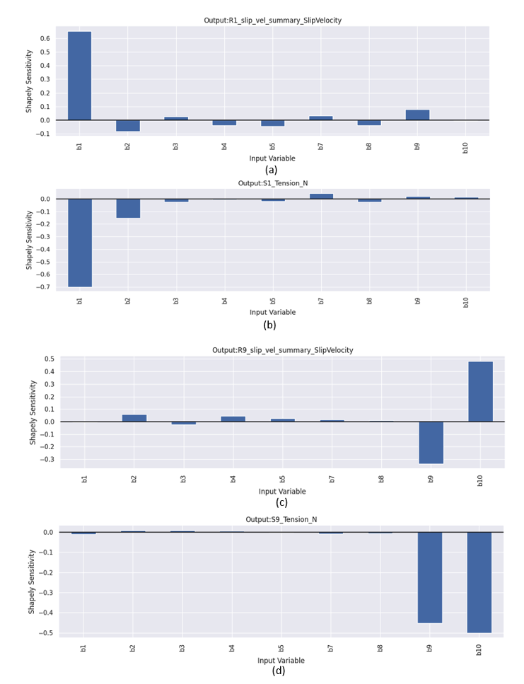
Figure 3 Example output of Shapley sensitivity analysis.

TwinFlow includes the TwinStat module which provides a library of algorithms and methods that are commonly used for probabilistic modeling for digital twins. In particular, TwinStat uses a Gaussian Kernel Density Estimator to produce the probability density distributions and cumulative density distributions for all outputs of the digital twin.

We gain further insights by reviewing the probability distributions for roller slip velocity and span tension. For example, Figure 4a show the probability density distribution of the R3 slip velocity obtained from the Monte Carlo sampling analysis where we varied the input damping coefficients. Figure 4b shows the cumulative distribution for the same data. The vertical dashed line indicates the slip velocity failure threshold and the probability curve crosses this threshold at approximately 90%, representing the probability of measurements being at or below the threshold.

We can tell that 90% of the cases have a slip velocity below the failure threshold of 1×10^-3 m/s, indicating that it’s unlikely that we’ll see roller slip at the R3 location. This suggests it might be feasible to forgo installation of a costly sensor in the R3 location.

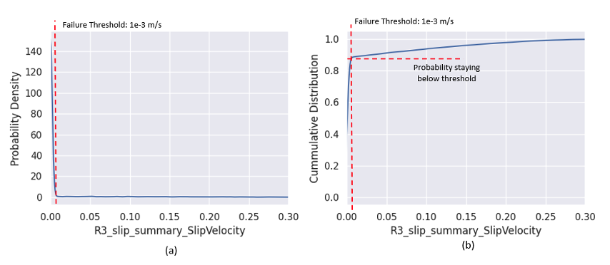
Figure 4 Probability of various slip velocities depending on changes in the roller viscous damping coefficients.

In contrast, Figure 5  shows that tension failures occur frequently for span 4. Figure 5b shows that only 38% of the cases remain below the tension failure threshold of 175 N. This means the probability of exceeding the failure threshold is 62% (calculated as 100% – 38%). The high failure rate suggests that we need to invest in the sensors to monitor span 4 tension.

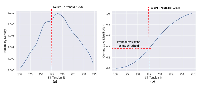
Figure 5 Probability of various slip velocities depending on changes in the roller viscous damping coefficients.

Performing similar analysis for all the roller slip velocities and span tensions reveals that spans 4,5,6 often exceed the tension failure threshold, but all other spans rarely or never fail. Similarly, rollers 1,5,6,7,8,9 often exceed the slip velocity failure threshold, but all other rollers rarely fail. This information alone already tells us which spans and rollers need monitoring with sensors, and which sensors we can remove or leave out.

Our goal is to minimize the cost of installing and maintaining sensors, while still being able to monitor the manufacturing process with sufficient resolution to minimize product defects. With this in mind, we note that angular velocity (RPM) sensors are much cheaper and less intrusive than tension load cells and linear velocity sensors.

The Shapley analysis provides cross-correlated sensitivities between potential sensors and each viscous damping coefficient. As our next step, we queried the dataset to generate the heatmap shown in Figure 6. A sensitivity heatmap like this visualizes the relationship between inputs and outputs of the digital twin. Green shades show a positive relationship – increasing the input increases the output. Red shades indicate a negative correlation – rising input values cause output values to decrease. The intensity of the color corresponds to the strength of the sensitivity. Higher saturation means the input has a larger effect on that output. Cells colored close to yellow have little to no sensitivity. Examining the heatmap reveals which input variables drive which outputs. Inputs that lack significant sensitivity to any outputs may represent opportunities to eliminate sensors to reduce costs.

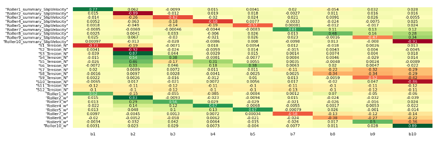
Figure 6 Heatmap of Shapley results

We can’t directly measure the damping coefficients in the system. Instead, we’ll use a combination of sensors with our digital twin to estimate the damping coefficients. The sensors provide data that allows for probabilistic inference with a digital twin for the damping coefficients. Once we have estimates for the damping coefficients, we can use them in the digital twin models to predict the values of other unmeasured variables in the system.

You’ll notice in Figure 6 that each sensor provides a different sensitivity and thus a different level of useful information. Some sensors can be strategically chosen due to either providing more information than other sensors, or information about multiple locations in the assembly line.

We know tension and linear velocity sensors are expensive so we are looking to see if RPM (“_w” in the table) can be used instead. For example, b1 exhibits sensitivity to “Roller1_w”, which also is sensitive to “S1_Tension” and “Roller1_Slip”, which means that “Roller1_w” should provide adequate information.

This analysis can reveal some non-intuitive results like that S5_Tension is more sensitive to b2 and b4 due to the blue nip roller pressure points in Figure 1. Doing these comparisons for all properties tells us that RPM should provide adequate information for all locations in the manufacturing line.

To verify the hypothesis that using lower-cost RPM sensors is as effective as the costlier slip velocity sensors/load cells, we used historical data with an Unscented Kalman Filter (available in TwinStat) to calibrate the Digital Twin. An Unscented Kalman Filter is a probabilistic Bayesian state estimation method that can be used to calibrate the model coefficients in our Level 4 Digital Twin. We showed this calibration approach in our earlier post discussing Level 4 DT setup and implementation.

We started by assuming installation of all 42 sensors, then used engineering analysis and customer feedback to determine that roller slip velocity and span tension are the critical quality parameters. This allowed us to reduce the number of sensors to 21. Shapley analysis then identified which specific rollers and spans were most failure-prone, enabling a further reduction to just 9 key sensors.

Finally, we substituted lower-cost RPM sensors for some slip velocity sensors and load cells, reducing cost while preserving monitoring capability. Through systematic evaluation we reduced 42 potential sensors down to 9 optimized, affordable sensors that will provide all the information we need to calibrate the Digital Twin, removing sensor redundancy.

Using Amazon Bedrock to augment traditional sensitivity analysis

The traditional manual approach to sensitivity analysis may be too time consuming or may include too many values to evaluate. Further data analysis techniques may be required such as using regressions on the data. However, as an experiment we decided to provide Amazon Bedrock with the Figure 6 data. In Figure 7 we presented this problem to the Claude 2.1 LLM model. Interestingly it correctly selected the RPM variables, but also concluded it would be possible to select a subset. The LLM model thinks it is possible to use fewer sensors than the human has selected to calibrate the digital twin. The LLM is attempting to take advantage of the fact that some viscous damping coefficients can potentially be used to predict multiple spans or roller properties. In a follow-up blog post, we will perform a more detailed exploration to assess the ability of using LLMs to assist with sensitivity analysis.

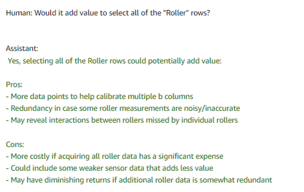
Figure 7 Comparison with Amazon Bedrock (Claude 2.1 Model). Note the raw data given to the LLM is not shown in the screenshots provided here.

AWS architecture

The AWS architecture used for the sensitivity study is depicted in Figure 8. Steps 1 – 3 are the same as described in the previous blog post for the Level 4 digital twin in which we install TwinFlow on an Amazon Elastic Compute Cloud (Amazon EC2) instance, setup a container which includes our MapleSim model, and push it up to Amazon ECR where the container is accessible to any AWS service.

We can also store the model in an Amazon Simple Storage Service (Amazon S3) bucket which will download the model when needed. This may be advantageous if we’re modifying the model for various studies.

When running a sensitivity study with TwinFlow (leveraging the TwinStat automation for sensitivity studies), it automatically sets up tables (creates the table and schema) within Amazon RDS (AWS SQL service). Based on user defined inputs and outputs in a JSON file, TwinFlow (leveraging the TwinStat automation) creates the input perturbation run list and executes in parallel all simulations using AWS Batch. AWS Batch is our cloud-native HPC scheduler that includes backend options for Amazon ECS, which is an AWS-specific container orchestrations service, AWS Fargate, which is a serverless execution option, and Amazon EKS which is our Kubernetes option.

We chose Amazon ECS because we wanted Amazon EC2 instances with larger numbers of CPUs than those available for Fargate. Fargate can create and deploy instances faster than ECS, however for tightly coupled numerical simulations often it’s better to scale up to minimize network latency thus minimizing runtime. Also, ECS enables fully-automated deployment unlike EKS. The specific Amazon EC2 instance type is automatically selected by AWS Batch auto-scaling based on the user-defined CPU/GPU and memory requirements.

Once all simulations have completed on AWS Batch, TwinStat downloads all data from the Amazon RDS tables and automatically performs the Shapley sensitivity study producing images of the probability distributions and sensitivity bar charts storing them in the local file system of the EC2 instance. A user then can review the results by downloading the images locally or store them in an Amazon S3 bucket for archiving.

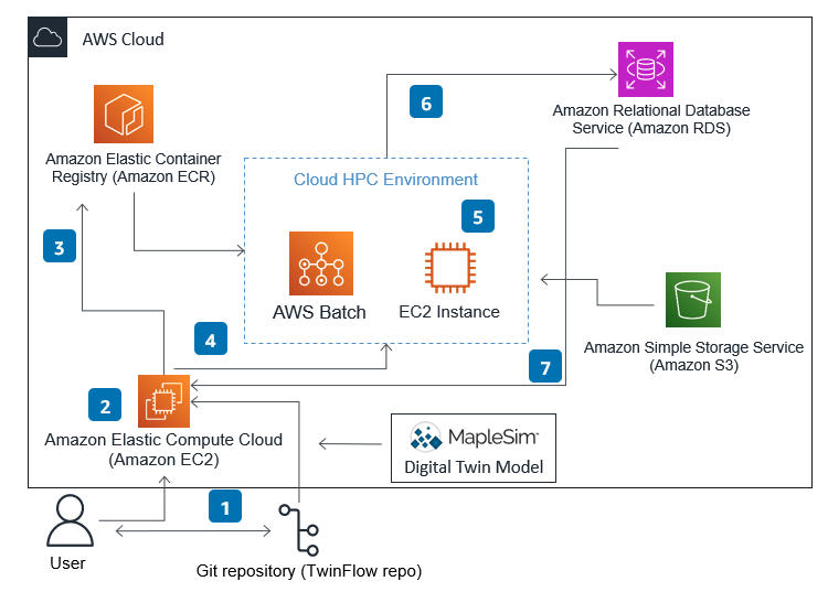
Figure 8 AWS cloud architecture used to perform sensitivity studies with our L4 Digital Twin

Summary

In this post, we showed how to perform a sensitivity analysis using a Digital Twin to identify the minimum set of sensors and sensor locations while maintaining effective monitoring of our roll-to-roll manufacturing process. MapleSim provides the physics-based model in the form of an FMU and TwinFlow allows us to run scalable number of scenarios on AWS, providing efficient and elastic computing resources.

In this Digital Twin example, the utility of a physics-based digital twin shows how we can quickly obtain actionable insights that directly impact business metrics. Digital twins are extremely versatile and can be leveraged at all phases of product development, from inception, implementation, to monitoring.

If you want to request a proof of concept or if you have feedback on the AWS tools, please reach out to us at ask-hpc@amazon.com.