AWS HPC Blog
Using a Level 4 Digital Twin for scenario analysis and risk assessment of manufacturing production on AWS
This post was contributed by Orang Vahid (Dir of Engineering Services) and Kayla Rossi (Application Engineer) at Maplesoft, and Ross Pivovar (Solution Architect) and Adam Rasheed (Snr Manager) from Autonomous Computing at AWS
One of the most common objectives for our Digital Twin (DT) customers is to use DTs for scenario analysis to assess risk and drive operational decisions. Customers want Digital Twins of their industrial facilities, production processes, and equipment to simulate different scenarios to optimize their operations and predictive maintenance strategies.
In a prior post, we described a four-level digital twin framework to help you understand these use cases and the technologies required to build them.
In this post today, we’re going to show you how to use an L4 Living Digital Twin for scenario analysis and operational decision support for a manufacturing line. We’ll use TwinFlow to combine a physics-based model created using MapleSim with probabilistic Bayesian methods to calibrate the L4 DT so it can adapt to the changing real-world conditions as the equipment degrades over time.
Then we’ll show you how to use the calibrated L4 DT to perform scenario analysis and risk assessment to simulate possible outcomes and make informed decisions. MapleSim provides the tools to create engineering simulation models of machine equipment and TwinFlow is an AWS open-source framework for building and deploying predictive models at scale.
L4 Living Digital Twin of roll-to-roll manufacturing
For our use case, we considered the web-handling process in roll-to-roll manufacturing for continuous materials like paper, film, and textiles. The web-handling process involves unwinding the material from a spool, guiding it through various treatments like printing or coating, and then winding it onto individual rolls. It’s essential that we precisely control the tension, alignment, and speed to ensure smooth processing and maintain product quality.
Figure 1 shows a schematic diagram of the web-handling equipment consisting of 9 rollers (labeled with “R”) and 12 material spans (labeled with “S”).
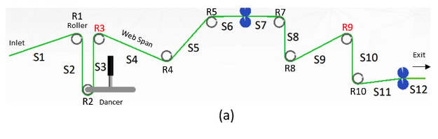
Figure 1 Schematic diagram of the web-handling equipment in which each span is labeled as S1 through S12 and rollers are label R1 through R10.
In our previous post, we showed you how to build and deploy L4 Digital Twin self-calibrating virtual sensors for predicting the tension in each of the spans and the slip velocity at each of the rollers throughout the web-handling process.
An L4 Living Digital Twin focuses on modeling the behavior of the physical system by updating the model parameters using real world observations. The capability to update the model is what makes it a “living” digital twin that’s synchronized with the physical system and continuously adapting as the physical system evolves. These situations are common in industrial facilities or manufacturing plants as equipment degrades over time. Examples of real-world observations include continuous data (time-series data from physical sensors), discrete measurements (discrete sensor measurements), or discrete observations (visual inspection data).
In this post, we’re extending our earlier example of L4 Digital Twin self-calibrating virtual sensors to conduct what-if scenario analysis predictions. Conceptually, an L4 Digital Twin forecast looks like Figure 2 which plots the predicted value over time. For our example, we focused on predicting the span tension within the material being manufactured. This is operationally important because tension failures occur when the tension within the material exceeds a threshold (175 Newtons in this example) resulting in product quality issues (e.g., scratches, breakage, wrinkling, or troughing).
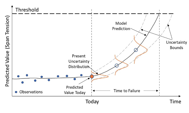
Figure 2 Conceptual plot showing historical measured data (observations) and L4 Digital Twin future forecast with uncertainty bounds showing when the predicted value will cross the failure threshold.
The vertical line (marked “Today”) shows the delineation between historical data collected in the past (the blue dots) and the future prediction with uncertainty bounds. In our case, the historical observations are values determined from the past inferred viscous damping coefficients because physical sensor measurements weren’t available. The L4 Digital Twin makes a prediction of the tension value today, and at all points in the future, including when the tension value will cross the damage threshold. The delta between Today and the time at which the prediction crosses the threshold represents the amount of time the operator has available to take some corrective action.
Of course, we can’t predict the future with perfect certainty so it’s important that all predictions be quantified with uncertainty bounds. This allows the operator to plan their corrective actions based on their risk tolerance. If the operator is risk averse, then they’d take corrective actions before the earliest uncertainty band crosses the threshold. In this way, they have a high probability of applying corrective action before failure happens. If they’re risk neutral, they would use the mean value. If they are willing to accept high risk, they could delay scheduling corrective actions to the later uncertainty band, recognizing that there’s a high probability of failure before they apply corrective actions. This last option may be logical when part replacement is more costly than lost production downtime.
In our example, we’re focusing on tension failure that results in a product quality issue, but the exact same approach can be used to predict equipment failure and remaining useful life (RUL) to proactively develop preventive maintenance plans.
Example scenario analysis
A potential scenario requiring risk assessment involves the detection of gradual dirt build-up on the roller bearings. Using the time series of the component degradation, we can predict when a failure could occur in the future. This knowledge lets us estimate when maintenance should be done.
The end result is that we can 1) maximize throughput of the manufacturing line to increase revenue and; 2) reduce costs by reducing defects and unnecessary downtime. A third benefit that’s rather application specific is a more targeted maintenance scheme. If we regularly schedule maintenance on all components, we run the risk of performing maintenance on components that don’t need servicing, increasing waste. Using a calibrated digital twin, we can specifically target the components that are degrading instead of everything at once.
To solidify these ideas, let’s think about the web-handling roll-to-roll manufacturing line again. Using the L4 Digital Twin we described in our last post lets us simulate a synthetic degradation scenario. In that scenario, we simulated bearing degradation by manually increasing the viscous damping coefficient for roller 9 from 0 on Day 15 to 0.2 on Day 19.
In Figure 3, we see the L4 Digital Twin is capturing that roller 9’s viscous damping coefficient is increasing from Day 15 to Day 19. We can tell that viscous damping is increasing, causing a change in tension in multiple spans, and we need to decide our course of action. The immediate risk to assess is whether we need to shut down the line to perform maintenance – or not.
Imagine that the dirt build up is detected on a Friday morning and the maintenance crew will be out on Monday because it’s a 3-day holiday weekend. Can we continue to generate product over the weekend and run the risk of increasing defects, or is it more cost effective to shut down the line for repairs on Friday before the maintenance crew heads home? Making this decision requires a forecast of the viscous damping coefficient and the span tension, and the uncertainty around these predictions. For example, predicting the damage threshold will be exceeded in 4 days ± 1 day means the maintenance can be deferred to Tuesday. If the prediction is 4 days ± 3 days, then it could very well be an issue tomorrow when the maintenance crew is out for the weekend.
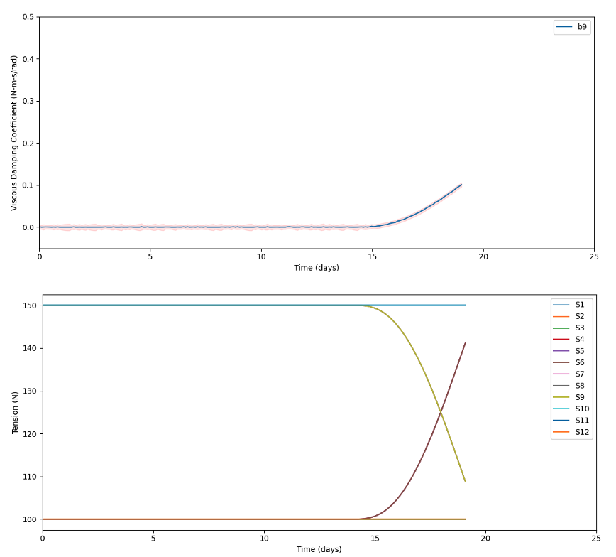
Figure 3 The inferred viscous damping coefficients calculated via TwinFlow UKF with MapleSim digital twin. Viscous damping coefficient of roller 9 is predicted to be increasing over the last several days
Using TwinFlow to perform scenario analysis
Like in our previous post, we first used MapleSim to create the physics-based model of the web-handling process and exported the model as a Modelica Functional Mockup Unit (FMU) which is an industry standard file format for simulation models.
We then used TwinFlow to combine the MapleSim model with an Unscented Kalman Filter (UKF) to infer the viscous damping coefficients of the rollers in the manufacturing line. This calibration process tunes the model based on the available physical sensor data (rotation speeds of the rollers). In that previous post, we showed how the self-calibrated virtual sensors then used the incoming sensor measurements (roller angular velocity and rotation speeds) to predict tension and slip velocity at any moment in time. Here, we’ll show how to use the same L4 Digital Twin to probabilistically forecast when the span tension will exceed the threshold. Readers can find this example described in an AWS Solution, and a full CDK deployment of the code used for this example up on Github with instructions about how to customize for your application and deploy it.
Using TwinFlow we combine the calibrated L4 Digital Twin with forecasting models to both predict when we’ll exceed the failure threshold – and the uncertainty associated with that prediction. There are a large variety of forecasting models that range from parametric models that work well on small data sets, to non-parametric deep-learning models that often require larger data sets and hyperparameter tuning.
For our application, we specifically want an estimate of the uncertainty in the forecast and a non-parametric method so that we don’t need to manually develop the model. A Gaussian Process (GP) is a natural fit for these requirements and a scalable low-code representation is available in TwinFlow. Using the historical time series data of the viscous damping coefficient, we can fit a GP to the data and forecast 4 days into the future along with the 95% uncertainty – as we’ve done in Figure 4.
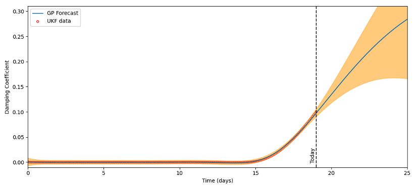
Figure 4 Forecast of viscous damping coefficient over next 4 days.
The uncertainty represents the prediction of possible future states for the viscous damping coefficients which we can then use with our L4 Digital Twin to forecast the span tension like in Figure 5. This figure corresponds to the conceptual diagram we drew in Figure 2 and you can tell that the tension crosses the threshold at 21.7 days with a lower uncertainty bound of 20.9 days. Given that today is Day 19, we can restate this as failure is expected in 2.7 days with an uncertainty lower bound of 1.9 days from today. We now have enough information to decide whether to shut down the manufacturing line for maintenance or not.
In our example, the operator notices a potential issue on Friday morning before the Monday long weekend. Our prediction is that failure will most likely occur after 2.7 days (Mon), but it could be as soon as 1.9 days (Sun) and the operator should preemptively perform the repair to avoid risking losing the weekend production. This type of analysis is very challenging for an operator to perform and the decision is often based on best judgement and operator experience. An additional benefit is that the L4 Digital Twin is modeling each component within the web-handling line – enabling the operator to identify which specific rollers are likely to require maintenance instead of spending time and money on all the rollers in the line.
![Figure 5 Plot showing historical measured data (observations) and L4 Digital Twin future forecast with uncertainty bounds showing when the tension will cross the failure threshold [175 N].](https://d2908q01vomqb2.cloudfront.net/e6c3dd630428fd54834172b8fd2735fed9416da4/2023/12/06/CleanShot-2023-12-06-at-13.06.07.png)
Figure 5 Plot showing historical measured data (observations) and L4 Digital Twin future forecast with uncertainty bounds showing when the tension will cross the failure threshold [175 N].
Figure 6 shows the forecast result at different time slices after being inserted into the digital twin. We can see that behavior is very non-linear with bimodal probability distributions, unlike the presumed normal (Gaussian) distributions shown in the conceptual diagram in Figure 2. We see the value of the L4 Digital Twin here because it’s impossible to know before-hand what the probability distributions would have been – and using the common assumption of Gaussian distributions would have resulted in inaccurate predictions.
The physical cause of this non-Gaussian distribution is the nature of the physics. The changing viscous damping coefficients can exhibit discontinuous changes in material slip, resulting in abrupt tension changes. This wouldn’t have been detected if we just used a data-only approach.
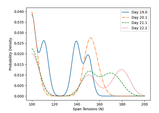
Figure 6 Probability density distributions for max span tension at different forecasted time slices.
AWS Architecture
The AWS architecture used for the L4 Digital Twin risk assessment is depicted in Figure 7. This architecture assumes the user has already enabled an L4 self-calibrating digital twin where the output of the previous architecture is being pushed into an AWS IoT SiteWise database. You can find a full CDK deployment of the code used for the example in this post on Github with instructions on how to customize for your application and deployment. In Figure 7, steps 1 – 3 are the same as the Level 4 digital twin.
With a small amount of code, we can use TwinFlow to pull down the IoT SiteWise data to an Amazon EC2 instance. We then fit a Gaussian Process (from the TwinStat module in TwinFlow) to the AWS IoT SiteWise data, forecast potential future outcomes, and then sampled the potential outcomes to obtain a data set to simulate with our digital twin.
Once we have a dataset, we can submit the different inputs to the cloud (step 4) like an on-premises HPC cluster. The main point of divergence from a standard on-premises HPC cluster is the requirement to containerize the application-specific code. AWS Batch is our cloud-native HPC scheduler that includes backend options for Amazon ECS, which is an AWS-specific container orchestrations service, AWS Fargate, which is a serverless execution option, and Amazon EKS which is our Kubernetes option. We used Amazon ECS because we wanted EC2 instances with large numbers of CPUs than those available for Fargate. Also, ECS enables fully-automated deployment unlike EKS.
TwinFlow reads a task list, or loads from memory, the various scenarios to be simulated. A container that includes the MapleSim digital twin and any application-specific automation is stored in a container within ECR for cloud access. The specific EC2 instance type is automatically selected by AWS Batch auto-scaling based on the user-defined CPU/GPU and memory requirements.
At step 5, the output predictions of the L4 DT simulations are generated with textual explanations and stored in an Amazon Simple Storage Service (Amazon S3) bucket which can then be made available to users via an interface. We can also store the prediction results in a database such as Amazon RDS (step 6), which can be pulled back into AWS IoT TwinMaker to compare with other data streams or review past forecasts for accuracy assessment.
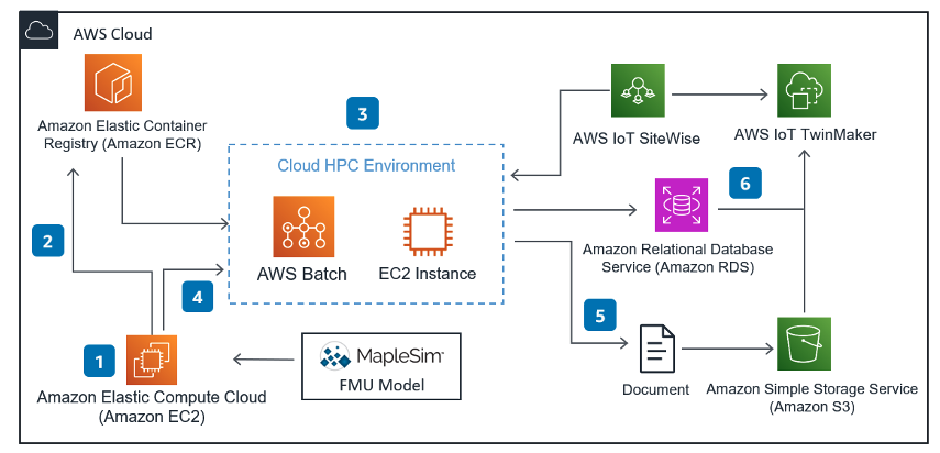
Figure 7 AWS cloud architecture needed to achieve digital twin periodic-calibration
Summary
In this post, we showed how to use a L4 Digital Twin to perform risk assessment and scenario analysis using an FMU model created by MapleSim. MapleSim provides the physics-based model in the form of an FMU and TwinFlow allows us to run scalable number of scenarios on AWS, providing efficient and elastic computing resources. In this L4 Digital Twin example the versatility of the hybrid modeling-based approach is demonstrated as the means of predicting fault scenarios that may have been missed if solely relying on physics-only or data-only based methods. Using the information gained from the scenario analysis enables you to do risk assessment and informed decision making.
If you want to request a proof of concept or if you have feedback on the AWS tools, please reach out to us at ask-hpc@amazon.com.
The content and opinions in this blog are those of the third-party author and AWS is not responsible for the content or accuracy of this blog.