Artificial Intelligence
Build a water consumption forecasting solution for a water utility agency using Amazon Forecast
Amazon Forecast is a fully managed service that uses machine learning (ML) to generate highly accurate forecasts, without requiring any prior ML experience. Forecast is applicable in a wide variety of use cases, including estimating supply and demand for inventory management, travel demand forecasting, workforce planning, and computing cloud infrastructure usage.
You can use Forecast to seamlessly conduct what-if analyses up to 80% faster to analyze and quantify the potential impact of business levers on your demand forecasts. A what-if analysis helps you investigate and explain how different scenarios might affect the baseline forecast created by Forecast. With Forecast, there are no servers to provision or ML models to build manually. Additionally, you only pay for what you use, and there is no minimum fee or upfront commitment. To use Forecast, you only need to provide historical data for what you want to forecast, and, optionally, any additional data that you believe may impact your forecasts.
Water utility providers have several forecasting use cases, but primary among them is predicting water consumption in an area or building to meet the demand. Also, it’s important for utility providers to forecast the increased consumption demand because of more apartments added in a building or more houses in the area. Predicting water consumption accurately is critical to avoid any service interruptions to the customer.
This post explores using Forecast to address this use case by using historical time series data.
Solution overview
Water is a natural resource and very critical to industry, agriculture, households, and our lives. Accurate water consumption forecasting is critical to make sure that an agency can run day-to-day operations efficiently. Water consumption forecasting is particularly challenging because demand is dynamic, and seasonal weather changes can have an impact. Predicting water consumption accurately is important so customers don’t face any service interruptions and in order to provide a stable service while maintaining low prices. Improved forecasting enables you to plan ahead to structure more cost-effective future contracts. The following are the two most common use cases:
- Better demand management – As a utility provider agency, you need to find a balance between water demand and supply. The agency collects information like number of people living in an apartment and number of apartments in a building before providing service. As a utility agency, you must balance aggregate supply and demand. You need to store sufficient water in order to meet the demand. Moreover, demand forecasting has become more challenging for the following reasons:
- The demand isn’t stable at all times and varies throughout the day. For example, water consumption at midnight is much less compared to in the morning.
- Weather can also have an impact on the overall consumption. For example, water consumption is higher in the summer than the winter in the northern hemisphere, and the other way around in the southern hemisphere.
- There is not enough rainfall or water storage mechanisms (lakes, reservoirs), or water filtering is insufficient. During the summer, demand can’t always keep up with supply. The water agencies have to forecast carefully to acquire other sources, which may be more expensive. Therefore, it’s critical for utility agencies to find alternative water sources like harvesting rainwater, capturing condensation from air handling units, or reclaiming wastewater.
- Conducting a what-if analysis for increased demand – Demand for water is rising due to multiple reasons. This includes a combination of population growth, economic development, and changing consumption patterns. Let’s imagine a scenario where an existing apartment building builds an extension and the number of households and people increase by a certain percentage. Now you need to do an analysis to forecast the supply for increased demand. This also helps you make a cost-effective contract for increased demand.
Forecasting can be challenging because you first need accurate models to forecast demand and then a quick and simple way to reproduce the forecast across a range of scenarios.
This post focuses on a solution to perform water consumption forecasting and a what-if analysis. This post doesn’t consider weather data for model training. However, you can add weather data, given its correlation to water consumption.
Prerequisites
Before getting started, we set up our resources. For this post, we use the us-east-1 Region.
- Create an Amazon Simple Storage Service (Amazon S3) bucket for storing the historical time series data. For instructions, refer to Create your first S3 bucket.
- Download data files from the GitHub repo and upload to the newly created S3 bucket.
- Create a new AWS Identity and Access Management (IAM) role. For instructions, see Set Up Permissions for Amazon Forecast. Be sure to provide the name of your S3 bucket.
Create a dataset group and datasets
This post demonstrates two use cases related to water demand forecast: forecasting the water demand based on past water consumption, and conducting a what-if analysis for increased demand.
Forecast can accept three types of datasets: target time series (TTS), related time series (RTS), and item metadata (IM). Target time series data defines the historical demand for the resources you’re predicting. The target time series dataset is mandatory. A related time series dataset includes time-series data that isn’t included in a target time series dataset and might improve the accuracy of your predictor.
In our example, the target time series dataset contains item_id and timestamp dimensions, and the complementary related time series dataset includes no_of_consumer. An important note with this dataset: the TTS ends on 2023-01-01, and the RTS ends on 2023-01-15. When performing what-if scenarios, it’s important to manipulate RTS variables beyond your known time horizon in TTS.
To conduct a what-if analysis, we need to import two CSV files representing the target time series data and the related time series data. Our example target time series file contains the item_id, timestamp, and demand, and our related time series file contains the product item_id, timestamp, and no_of consumer.
To import your data, complete the following steps:
- On the Forecast console, choose View dataset groups.

- Choose Create dataset group.

- For Dataset group name, enter a name (for this post,
water_consumption_datasetgroup). - For Forecasting domain, choose a forecasting domain (for this post, Custom).
- Choose Next.

- On the Create target time series dataset page, provide the dataset name, frequency of your data, and data schema.

- On the Dataset import details page, enter a dataset import name.
- For Import file type, select CSV and enter the data location.
- Choose the IAM role you created earlier as a prerequisite.
- Choose Start.

You’re redirected to the dashboard that you can use to track progress.
- To import the related time series file, on the dashboard, choose Import.

- On the Create related time series dataset page, provide the dataset name and data schema.

- On the Dataset import details page, enter a dataset import name.
- For Import file type, select CSV and enter the data location.
- Choose the IAM role you created earlier.
- Choose Start.

Train a predictor
Next, we train a predictor.
- On the dashboard, choose Start under Train a predictor.

- On the Train predictor page, enter a name for your predictor.
- Specify how long in the future you want to forecast and at what frequency.
- Specify the number of quantiles you want to forecast for.
Forecast uses AutoPredictor to create predictors. For more information, refer to Training Predictors.
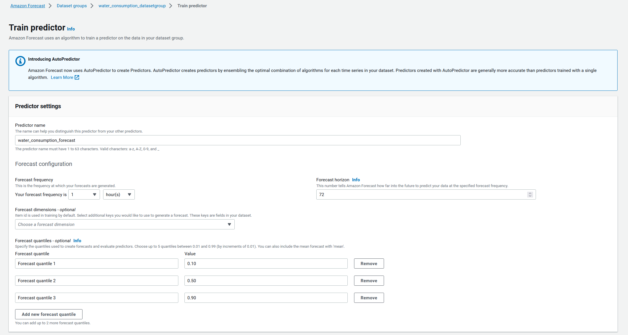
- Choose Create.
Create a forecast
After our predictor is trained (this can take approximately 3.5 hours), we create a forecast. You will know that your predictor is trained when you see the View predictors button on your dashboard.
- Choose Start under Generate forecasts on the dashboard.

- On the Create a forecast page, enter a forecast name.
- For Predictor, choose the predictor that you created.
- Optionally, specify the forecast quantiles.
- Specify the items to generate a forecast for.
- Choose Start.

Query your forecast
You can query a forecast using the Query forecast option. By default, the complete range of the forecast is returned. You can request a specific date range within the complete forecast. When you query a forecast, you must specify filtering criteria. A filter is a key-value pair. The key is one of the schema attribute names (including forecast dimensions) from one of the datasets used to create the forecast. The value is a valid value for the specified key. You can specify multiple key-value pairs. The returned forecast will only contain items that satisfy all the criteria.
- Choose Query forecast on the dashboard.

- Provide the filter criteria for start date and end date.
- Specify your forecast key and value.
- Choose Get Forecast.

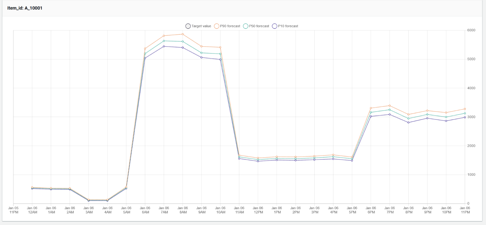
The following screenshot shows the forecast energy consumption for the same apartment (item ID A_10001) using the forecast model.
Create a what-if analysis
At this point, we have created our baseline forecast can now conduct a what-if analysis. Let’s imagine a scenario where an existing apartment building adds an extension, and the number of households and people increases by 20%. Now you need to do an analysis to forecast increased supply based on increased demand.
There are three stages to conducting a what-if analysis: setting up the analysis, creating the what-if forecast by defining what is changed in the scenario, and comparing the results.
- To set up your analysis, choose Explore what-if analysis on the dashboard.

- Choose Create.

- Enter a unique name and choose the baseline forecast.
- Choose the items in your dataset you want to conduct a what-if analysis for. You have two options:
- Select all items is the default, which we choose in this post.
- If you want to pick specific items, choose Select items with a file and import a CSV file containing the unique identifier for the corresponding item and any associated dimensions.
- Choose Create what-if analysis.

Create a what-if forecast
Next, we create a what-if forecast to define the scenario we want to analyze.
- In the What-if forecast section, choose Create.

- Enter a name of your scenario.
- You can define your scenario through two options:
- Use transformation functions – Use the transformation builder to transform the related time series data you imported. For this walkthrough, we evaluate how the demand for an item in our dataset changes when the number of consumers increases by 20% when compared to the price in the baseline forecast.
- Define the what-if forecast with a replacement dataset – Replace the related time series dataset you imported.
For our example, we create a scenario where we increase no_of_consumer by 20% applicable to item ID A_10001, and no_of_consumer is a feature in the dataset. You need this analysis to forecast and meet the water supply for increased demand. This analysis also helps you make a cost-effective contract based on the water demand forecast.
- For What-if forecast definition method, select Use transformation functions.
- Choose Multiply as our operator, no_of_consumer as our time series, and enter 1.2.
- Choose Add condition.
- Choose Equals as the operation and enter A_10001 for item_id.
- Choose Create.

Compare the forecasts
We can now compare the what-if forecasts for both our scenarios, comparing a 20% increase in consumers with the baseline demand.
- On the analysis insights page, navigate to the Compare what-if forecasts section.
- For item_id, enter the item to analyze (in our scenario, enter
A_10001). - For What-if forecasts, choose
water_demand_whatif_analyis. - Choose Compare what-if.

- You can choose the baseline forecast for the analysis.
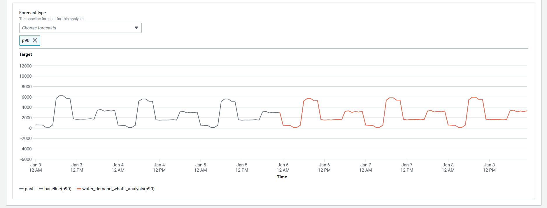
The following graph shows the resulting demand for our scenario. The red line shows the forecast of future water consumption for 20% increased population. The P90 forecast type indicates the true value is expected to be lower than the predicted value 90% of the time. You can use this demand forecast to effectively manage water supply for increased demand and avoid any service interruptions.
Export your data
To export your data to CSV, complete the following steps:
- Choose Create export.

- Enter a name for your export file (for this post,
water_demand_export). - Specify the scenarios to be exported by selecting the scenarios on the What-If Forecast drop-down menu.
You can export multiple scenarios at once in a combined file.
- For Export location, specify the Amazon S3 location.
- To begin the export, choose Create Export.

- To download the export, navigate to S3 file path location on the Amazon S3 console, select the file, and choose Download.
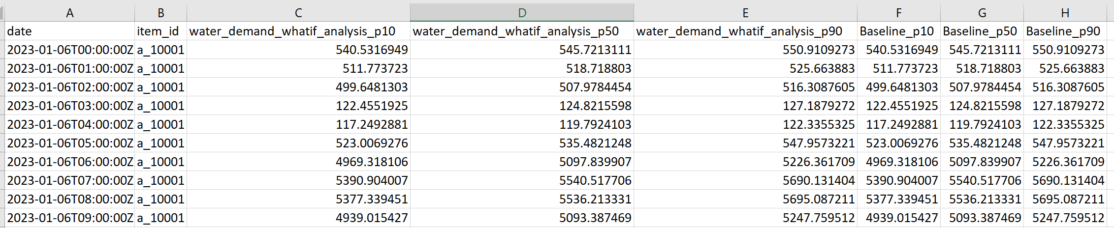
The export file will contain the timestamp, item_id, and forecasts for each quantile for all scenarios selected (including the base scenario).
Clean up the resources
To avoid incurring future charges, remove the resources created by this solution:
- Delete the Forecast resources you created.
- Delete the S3 bucket.
Conclusion
In this post, we showed you how easy to use how to use Forecast and its underlying system architecture to predict water demand using water consumption data. A what-if scenario analysis is a critical tool to help navigate through the uncertainties of business. It provides foresight and a mechanism to stress-test ideas, leaving businesses more resilient, better prepared, and in control of their future. Other utility providers like electricity or gas providers can use Forecast to build solutions and meet utility demand in a cost-effective way.
The steps in this post demonstrated how to build the solution on the AWS Management Console. To directly use Forecast APIs for building the solution, follow the notebook in our GitHub repo.
We encourage you to learn more by visiting the Amazon Forecast Developer Guide and try out the end-to-end solution enabled by these services with a dataset relevant to your business KPIs.
About the Author
 Dhiraj Thakur is a Solutions Architect with Amazon Web Services. He works with AWS customers and partners to provide guidance on enterprise cloud adoption, migration, and strategy. He is passionate about technology and enjoys building and experimenting in the analytics and AI/ML space.