Perform a large-scale principal component analysis faster using Amazon SageMaker

In this blog post, we conduct a performance comparison for PCA using Amazon SageMaker, Spark ML, and Scikit-Learn on high-dimensional datasets. SageMaker consistently showed faster computational performance. Refer Figures (1) and (2) at the bottom to see the speed improvements.

Principal Component Analysis

Principal Component Analysis (PCA) is an unsupervised learning algorithm that attempts to reduce the dimensionality (e.g., number of features) within a dataset while still retaining as much information as possible. PCA linearly transforms a data matrix into an orthogonal space, where the columns are now independent of one another and each column can account for a known proportion of variance in the data. In other words, it finds a new set of features called components, which are composites of the original features such that they are uncorrelated to one another. They are also constrained so that the first component accounts for the largest possible variability in the data, the second component the second most variability, and so on.

For a more comprehensive description please refer to https://docs.aws.amazon.com/sagemaker/latest/dg/how-pca-works.html.

PCA is powerful, both as a tool for Exploratory Data Analysis (EDA) and as an algorithm for machine learning (ML). For EDA, PCA is optimal for dimensionality reduction and reducing the multi-collinearity of a data problem. As a ML methodology, PCA can be combined with others ML methodologies to improve their effectiveness in anomaly detection (e.g., identifying suspicious traffic in networks), robust forecasting (e.g., quantitative finance), and classification (e.g., credit scoring), to name a few.

Advancements in technology have led to increased capabilities in data collection, leading to data sets of larger sizes and of more granular detail. PCA is a tremendously useful ML tool for big data analysis. However, PCA is not easily parallelizable, and until Amazon SageMaker, has not been as scalable for practical use in big data applications.

In this blog post, we’ll demonstrate the speed and scalability of the Amazon SageMaker PCA function. For matrices of increasing size, we will measure the Amazon SageMaker PCA runtime against those of Spark ML’s and Scikit-Learn’s PCA functions.

Amazon SageMaker

Amazon SageMaker is a fully-managed platform from AWS that enables developers and data scientists to quickly and easily build, train, and deploy machine learning models at any scale. Amazon SageMaker removes the barriers that typically slow down developers who want to use machine learning. Amazon SageMaker has some built-in algorithms, such as linear learner, k-means, DeepAR, PCA, and others.

Datasets

To demonstrate the scalability of the Amazon SageMaker PCA, we have chosen a large real-world data set, and we have simulated even larger data sets to be four times the number of observations as the real-world data set, and up to twice the number of features.

Real data set: NIPS Bag of Words

This data set is the distribution of words in the full texts of NIPS conference papers that were published from 1987 to 2015, in the form of an 11,463-by-5,812 matrix of word counts [Perrone et al., 2016]. Each column represents a corresponding NIPS paper and contains the number of times each of the 11,463 words appeared in that paper. The names of the columns identify the corresponding NIPS document by the format PublicationYear_PaperID, for a total of 5,812 documents. This data set is publicly available at https://archive.ics.uci.edu/ml/datasets/NIPS+Conference+Papers+1987-2015#.

Analysis on such a dataset could, for example, provide insight into which keywords increase the likelihood of a publication, or would lead to a higher number of citations.

Simulated data sets

Our simulated data sets are composed of 20k observations, and consist of 5k, 10k, 15k, and 20k features respectively.

Code: PCA implementation using Amazon SageMaker

We created a ml.m4.xlarge SageMaker notebook instance with a Conda MXNet kernel. We include the line numbers of our code that correspond to each step for the implementation’s reproducibility. Our code is a self-contained working Sage-Maker notebook that you can download from here.

Let’s download the NIPS data set. We transpose the matrix, so that columns represent words and rows represent documents. This results in a 5812-by-11463 matrix. Check that the indices, that is, the strings of document IDs, are not included as a superfluous column. We ingest our matrix as binary stream file object.

# Download NIPS data set and transpose matrix.
import sys
!wget https://archive.ics.uci.edu/ml/machine-learning-databases/00371/NIPS_1987-2015.csv
filename = 'NIPS_1987-2015.csv'
import pandas as pd
data = pd.read_csv('NIPS_1987-2015.csv', index_col=0)


# Convert data to binary stream.
matrx = data.transpose().apply(lambda x: (x-x.mean())/x.std()).as_matrix()
import io
import sagemaker.amazon.common as smac
buf = io.BytesIO()
smac.write_numpy_to_dense_tensor(buf, matrx)
buf.seek(0)

Now we are ready to upload the file object to our Amazon S3 bucket. We specify two paths: one to where our uploaded matrix will reside, and one to where Amazon SageMaker will write the output. Amazon SageMaker will create any folders within the paths that do not already exist.

# Specify S3 file paths for training data and for output location. Upload data to S3.
import boto3
bucket = '<your-bucket-name>'
prefix = 'sagemaker/pca-nips'
key = 'NIPS-bytes-data'

import os
s3_train_data = 's3://{}/{}/train/{}'.format(bucket, prefix, key)
boto3.resource('s3').Bucket(bucket).Object(os.path.join(prefix, 'train', key)).upload_fileobj(buf)
print('uploaded training data location: {}'.format(s3_train_data))

output_location = 's3://{}/{}/output'.format(bucket, prefix)
print('training artifacts will be uploaded to: {}'.format(output_location))

Instantiating a PCA session of Amazon SageMaker requires six arguments. The first one is the container address corresponding to the Region in which our SageMaker notebook resides; e.g., us-east-1 has container 382416733822.dkr.ecr.us-east-1.amazonaws.com/pca:latest. The second is the Amazon SageMaker IAM role, which was created in conjunction with the creation of this notebook.  For the third and fourth arguments, we are specifying one train_instance_count of train_instance_type ml.c4.8xlarge as the virtual environment in which to run our PCA. In actuality, we recommend a GPU machine, such as ml.p2.xlarge or ml.p3.xlarge, since for example, the ml.p2.xlarge is less expensive than a ml.c4.8xlarge and finishes the job in less time. Here we have chosen the ml.c4.8xlarge instance for its large number of cores and high memory, and for fairness, use this same machine type across the experiment. The fifth argument is the path we defined earlier for output to be written. Lastly, pass the Amazon SageMaker session itself.

# Lookup container address per AWS region.
containers = {'us-west-2': '174872318107.dkr.ecr.us-west-2.amazonaws.com/pca:latest',
              'us-east-1': '382416733822.dkr.ecr.us-east-1.amazonaws.com/pca:latest',
              'us-east-2': '404615174143.dkr.ecr.us-east-2.amazonaws.com/pca:latest',
              'eu-west-1': '438346466558.dkr.ecr.eu-west-1.amazonaws.com/pca:latest'}

# Get SageMaker IAM execution role.
from sagemaker import get_execution_role
role = get_execution_role()

# Create SageMaker session. 
import sagemaker
sess = sagemaker.Session()

# Instantiate SageMaker PCA with six arguments.                                              
pca = sagemaker.estimator.Estimator(containers[boto3.Session().region_name],
                                    role,
                                    train_instance_count=2,
                                    train_instance_type='ml.c4.8xlarge',
                                    output_path=output_location,
                                    sagemaker_session=sess)

Thus far, we have specified the Amazon SageMaker training instance parameters. We still want to specify the hyper-parameters for the PCA algorithm. The hyper-parameters are:  the number of features, the desired number of principal components to return, a Boolean to subtract each column’s mean prior to matrix decomposition, whether to perform `regular’ or `randomized’ PCA, and lastly, the mini-batch size.

# Specify PCA hyper-parameters 
import numpy as np
pca.set_hyperparameters(feature_dim=np.shape(matrx)[1],
                        num_components= np.shape(matrx)[1]-1,
                        subtract_mean=True,
                        algorithm_mode='regular',
                        mini_batch_size=200)

Now we simply kick off the PCA fitting, with our Amazon S3 data path passed as the input. Amazon SageMaker writes a log file for each job to an S3 location of the following format:

https://console.aws.amazon.com/cloudwatch/home?region=<region> #logEventViewer:group=/aws/sagemaker/TrainingJobs;stream=<algo-YYYY-MM-DD-hh-mm-ss-SSS>/algo-<int>-<timestamp>

The logs discern between how long the instances take to spin up and how long the PCA fit takes.  Unlike when you use on-premises machines, you do not pay for provisioning time, only for consumption. We found the specified instance takes approximately 7 minutes to be provisioned. Once the instances are ready, the PCA is fit, and the output is written to the given S3 location as a compressed tar file.

# Kick-off PCA fitting.
import time 
pca.fit({'train': s3_train_data})

Let’s download the tarred output, the contents of which can be read as an MXNet ndarray. The ndarray has three attributes: mean, an array of column means; s, an ndarray of singular values; and v, an ndarray of principal component vectors.

# Download and unpack returned PCA model artifact. 
job_name = pca.latest_training_job.name
os.system('aws s3 cp {}/{}/output/model.tar.gz ./'.format(output_location, job_name)) 
!tar xzvf model.tar.gz

import mxnet as mx
pca_model = mx.ndarray.load('model_algo-1')
mean = pca_model['mean']
singular_values = np.sort(pca_model['s'].asnumpy())[::-1]
pc_vectors = pca_model['v']

Performance evaluation against other tools: SparkML and Scikit-Learn

We recognize Spark ML and Scikit-Learn as the top two open-source libraries currently attempting to address large-scale PCA.

Spark is a cluster-computing framework that has a distributed machine learning library equipped with common statistical algorithms, and it has been benchmarked at nine times faster than disk-based implementation [Rocha et al., 2017]. Scikit-Learn is a machine learning library developed for the Python programming language. Although it was initially designed for single machine uses, specific implementations of its PCA have been parallelized [Pedregosa et al., 2011].

We spun up identical c4.8xlarge instances for each environment and proceeded to record the PCA runtimes for increasing dimensionality, on both the real-world NIPS data and on our simulated data.

Results

Figure 1 shows that for matrices of up to 1000 features, Spark ML performs PCA approximately 90x more slowly than Amazon SageMaker. Above 5000 features, Spark ML is prohibitively time-consuming and therefore is excluded from higher-dimensional comparison in this blog post.

Table 1: Matrix dimensionalities per PCA test case

For low dimensional matrices, the performance of Scikit-Learn’s PCA is on par with that of Amazon SageMaker. Figure 1 shows that only when approaching a matrix of 5000 features, does SageMaker see a 5x advantage over Scikit-Learn. However, it is very important to note here, that that Scikit-Learn does not perform a complete PCA on non-square matrices. The maximum number of components Scikit-Learn will return is equal to min(num_observations; num_features). In other words, Scikit-Learn drops remaining observations when num_observations exceeds num_features. So, the runtimes seen here are for truncated smaller sized matrices.

In addition to limiting Scikit-Learn’s usefulness in analytical applications, it also limits our ability for side-by-side time trials. We turn to our simulated data sets, where the feature dimensionality never exceeds the sample size. Figure 2 shows that the Amazon SageMaker PCA performs about 5x faster than that of Scikit-Learn.

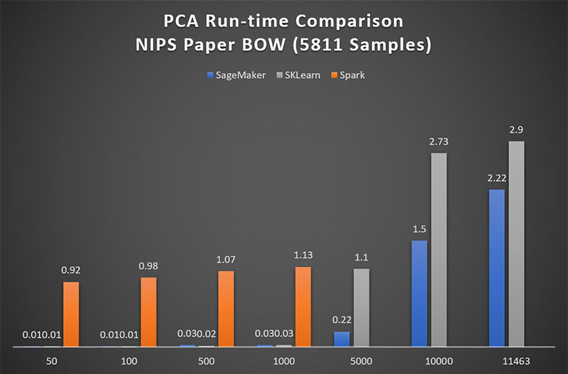
Figure 1: Amazon SageMaker achieves 90x performance over Spark

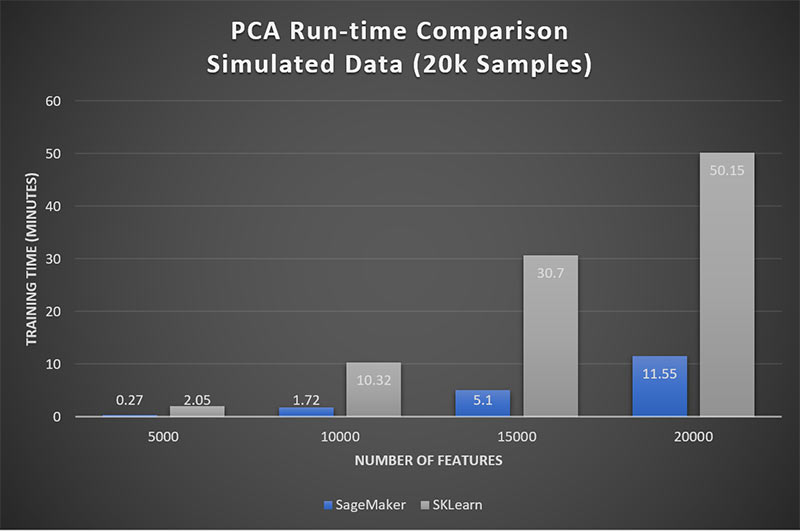
Figure 2: Amazon SageMaker achieves 5x performance over Scikit-Learn

Conclusion

PCA has always been important in low-dimensional problems for data visualization and data decorrelation. However, as real-world problems are dealing with increasingly large data sets, scalable PCA for high-dimensional problems is more important than ever. In this blog post we demonstrated the advantages Amazon SageMaker provides in achieving the most scalable framework for PCA.

The code shown here is completely self-contained. To get started, open a SageMaker notebook and copy and paste the blocks of our code to replicate the NIPS results seen here. Or, download this notebook with the code blocks pre-filled. This serverless tool will handle the underlying platform and computing framework. Try out a range of requested number of components and see how Amazon SageMaker scales.  You can also try the code on your own data set with differing numbers of observations and features.

References

[Pedregosa et al., 2011] Pedregosa, F., Varoquaux, G., Gramfort, A., Michel, V., Thirion, B., Grisel, O., Blondel, M., Prettenhofer, P., Weiss, R., Dubourg, V., Vanderplas, J., Passos, A., Cournapeau, D., Brucher, M., Perrot, M., and Duchesnay, E. (2011). Scikit-learn: Machine learning in Python. Journal of Machine Learning Research, 12:2825{2830. 4

[Perrone et al., 2016] Perrone, V., Jenkins, P. A., Spano, D., and Teh, Y. W. (2016). Poisson random fields for dynamic feature models. arXiv preprint arXiv:1611.07460. 2

[Rocha et al., 2017] Rocha, A., Correia, A. M., Adeli, H., Reis, L. P., and Costanzo, S. (2017). Recent Advances in Information Systems and Technologies, volume 3. Springer. 4

About the Authors

Elena Ehrlich is a Data Scientist with AWS Professional Services. She has a PhD in Mathematics from Imperial College London and has worked across industries including defense, finance, and ad tech. Today she is working with customers to develop and integrate machine learning and AI solutions on AWS.

Hanif Mahboobi is a Data Scientist with AWS Professional Services. He received his PhD from Sharif University of Technology in 2009 and has several years of experience as a researcher in scientific computing, complex systems’ modeling and data science. Currently, he helps AWS customers across different industries to develop machine learning and artificial intelligence solutions.