Amazon SageMaker now supports PyTorch and TensorFlow 1.8

Starting today, you can easily train and deploy your PyTorch deep learning models in Amazon SageMaker. This is the fourth deep learning framework that Amazon SageMaker has added support for, in addition to TensorFlow, Apache MXNet, and Chainer. Just like with those frameworks, now you can write your PyTorch script like you normally would and rely on Amazon SageMaker training to handle setting up the distributed training cluster, transferring data, and even hyperparameter tuning. On the inference side, Amazon SageMaker provides a managed, highly available, online endpoint that can be automatically scaled up as needed.

In addition to PyTorch, we’re also adding the latest stable versions of TensorFlow (1.7 and 1.8), allowing you to start taking advantage of new features in these versions such as tf.custom_gradient and the pre-made BoostedTree estimators today. The Amazon SageMaker TensorFlow estimator is setup to use the latest version by default, so you don’t even need to update your code.

Supporting many deep learning frameworks is important to developers, since each of the deep learning frameworks has unique areas of strength. PyTorch is a framework used heavily by deep learning researchers, but it is also rapidly gaining popularity among developers due its flexibility and ease of use. TensorFlow is well established and continues to add great features with each release. We’ll continue to invest in these, and other popular engines such as MXNet and Chainer.

PyTorch in Amazon SageMaker

The PyTorch framework is unique. It differs from other frameworks, such as TensorFlow, MXNet, Caffe, etc., because it uses a technique called reverse-mode auto-differentiation, which allows you to build neural networks dynamically. It is also deeply integrated with Python, allowing you to use typical Python control flows in your networks or to write new network layers using Cython, Numba, NumPy, etc. Finally, PyTorch is fast, with support for acceleration libraries like MKL, CuDNN, and NCCL. It recently posted wins in the DAWNBench Competition from the team at fast.ai using PyTorch.

Using PyTorch in Amazon SageMaker is as easy as using the other pre-built deep learning containers. Just provide your training or hosting script, which consists of standard PyTorch wrapped in a few helper functions, and then use the PyTorch estimator from the Amazon SageMaker Python SDK as follows:

estimator = PyTorch(entry_point="pytorch_script.py",
                    role=role,
                    train_instance_count=2,
                    train_instance_type='ml.p2.xlarge',
                    hyperparameters={'epochs': 10,
                                     'lr': 0.01})

Feel free to see our example notebooks, documentation, or follow along with the below example for more detail.

Training and deploying a neural network with PyTorch

For this example we’ll fit a straightforward convolutional neural network on the MNIST handwritten digits dataset. This consists of 70,000 labeled 28×28 pixel grayscale images (60,000 for training, 10,000 for testing) with 10 classes (one for each digit from 0 to 9). The Amazon SageMaker PyTorch container uses script mode, which expects the input script in a format that should be close to what you’d run outside of SageMaker. Let’s start by looking at that code. The full file is based on PyTorch’s own MNIST example, with the addition of distributed training. We’ll just highlight the most important pieces.

Entry point script

Starting with the main guard, we’ll use a parser to read in hyperparameters that we pass to our Amazon SageMaker estimator when creating the training job. The hyperparameters will be made available as arguments to our input script in the training container. Here, we look for hyperparameters like batch size, epochs, learning rate, momentum, etc. If we don’t define their values in our SageMaker estimator call, they’ll take on the defaults we’ve provided. We also use the training_env() method from the custom sagemaker_containers library, which provides container specifics like training and model directories and instance configurations. You can also access them through specific environment variables. For more information, please visit SageMaker Containers GitHub repository.

if __name__ == '__main__':
    parser = argparse.ArgumentParser()

    # Data and model checkpoints directories
    parser.add_argument('--batch-size', type=int, default=64, metavar='N',
                        help='input batch size for training (default: 64)')
    parser.add_argument('--test-batch-size', type=int, default=1000, metavar='N',
                        help='input batch size for testing (default: 1000)')
    parser.add_argument('--epochs', type=int, default=10, metavar='N',
                        help='number of epochs to train (default: 10)')
    parser.add_argument('--lr', type=float, default=0.01, metavar='LR',
                        help='learning rate (default: 0.01)')
    parser.add_argument('--momentum', type=float, default=0.5, metavar='M',
                        help='SGD momentum (default: 0.5)')
    parser.add_argument('--seed', type=int, default=1, metavar='S',
                        help='random seed (default: 1)')
    parser.add_argument('--log-interval', type=int, default=100, metavar='N',
                        help='how many batches to wait before logging training status')
    parser.add_argument('--backend', type=str, default=None,
                        help='backend for distributed training (tcp, gloo on cpu and gloo, nccl on gpu)')

    # Container environment
    env = sagemaker_containers.training_env()
    parser.add_argument('--hosts', type=list, default=env.hosts)
    parser.add_argument('--current-host', type=str, default=env.current_host)
    parser.add_argument('--model-dir', type=str, default=env.model_dir)
    parser.add_argument('--data-dir', type=str,
                        default=env.channel_input_dirs['training'])
    parser.add_argument('--num-gpus', type=int, default=env.num_gpus)

    train(parser.parse_args())

After we’ve defined our hyperparameters, we pass them to our train() function, which we also define in our input script. The train() function takes on several tasks. First, it sets up resources properly (GPU, distributed compute, etc.).

def train(args):
    is_distributed = len(args.hosts) > 1 and args.backend is not None
    logger.debug("Distributed training - {}".format(is_distributed))
    use_cuda = args.num_gpus > 0
    logger.debug("Number of gpus available - {}".format(args.num_gpus))
    kwargs = {'num_workers': 1, 'pin_memory': True} if use_cuda else {}
    device = torch.device("cuda" if use_cuda else "cpu")

    if is_distributed:
        # Initialize the distributed environment.
        world_size = len(args.hosts)
        os.environ['WORLD_SIZE'] = str(world_size)
        host_rank = args.hosts.index(args.current_host)
        dist.init_process_group(backend=args.backend, 
                                rank=host_rank, 
                                world_size=world_size)
        logger.info(
            'Init distributed env: \'{}\' backend on {} nodes. '.format(args.backend, 
                dist.get_world_size()) + \
            'Current host rank is {}. Number of gpus: {}'.format(
                dist.get_rank(), args.num_gpus))

    # set the seed for generating random numbers
    torch.manual_seed(args.seed)
    if use_cuda:
        torch.cuda.manual_seed(args.seed)

    ...

Then, it loads our datasets.

    ...
    
    train_loader = _get_train_data_loader(args.batch_size, 
                                          args.data_dir, 
                                          is_distributed,
                                          **kwargs)
    test_loader = _get_test_data_loader(args.test_batch_size, 
                                        args.data_dir,
                                        **kwargs)

    ...

And it initiates our network, model, and optimizer.

    ...

    model = Net().to(device)
    if is_distributed and use_cuda:
        # multi-machine multi-gpu case
        model = torch.nn.parallel.DistributedDataParallel(model)
    else:
        # single-machine multi-gpu case or single-machine or multi-machine cpu case
        model = torch.nn.DataParallel(model)

    optimizer = optim.SGD(model.parameters(), lr=args.lr, momentum=args.momentum)
    
    ...

Next, it loops through epochs to train the network. Here we loop through mini-batches, use back-propagation to minimize the model’s negative log likelihood loss, evaluate training loss every 100 mini-batches, and finally evaluate test loss at the end of each epoch.

    ...
    
    for epoch in range(1, args.epochs + 1):
        model.train()
        for batch_idx, (data, target) in enumerate(train_loader, 1):
            data, target = data.to(device), target.to(device)
            optimizer.zero_grad()
            output = model(data)
            loss = F.nll_loss(output, target)
            loss.backward()
            if is_distributed and not use_cuda:
                # average gradients manually for multi-machine cpu case only
                _average_gradients(model)
            optimizer.step()
            if batch_idx % args.log_interval == 0:
                logger.info('Train Epoch: {} [{}/{} ({:.0f}%)] Loss: {:.6f}'.format(
                    epoch, batch_idx * len(data), len(train_loader.sampler),
                    100. * batch_idx / len(train_loader), loss.item()))
        test(model, test_loader, device)

    ...

And finally, we save our model.

    ...
    
    save_model(model, args.model_dir)

We used a number of helper functions and classes within train(). This includes _get_train_data_loader() and _get_test_data_loader() which reads in shuffled mini-batches of our MNIST data, converts the 28×28 matrices to PyTorch tensors, and normalizes the pixel values.

def _get_train_data_loader(batch_size, training_dir, is_distributed, **kwargs):
    logger.info("Get train data loader")
    dataset = datasets.MNIST(training_dir, 
                             train=True, 
                             transform=transforms.Compose([
                                 transforms.ToTensor(),
                                 transforms.Normalize((0.1307,), (0.3081,))]))
    if is_distributed:
        train_sampler = torch.utils.data.distributed.DistributedSampler(dataset)
    else:
        train_sampler = None
    return torch.utils.data.DataLoader(dataset, 
                                       batch_size=batch_size, 
                                       shuffle=train_sampler is None,
                                       sampler=train_sampler,
                                       **kwargs)


def _get_test_data_loader(test_batch_size, training_dir, **kwargs):
    logger.info("Get test data loader")
    dataset = datasets.MNIST(training_dir, 
                             train=False, 
                             transform=transforms.Compose([
                                 transforms.ToTensor(),
                                 transforms.Normalize((0.1307,), (0.3081,))]))
    return torch.utils.data.DataLoader(dataset,
                                       batch_size=test_batch_size, 
                                       shuffle=True,
                                       **kwargs)

We also have the Net class that defines our network architecture and what a forward pass through the network means. In this case, it’s two convolutional and max pooling layers with rectified linear unit (ReLU) activation, followed by a two fully connected layers with dropout intermixed.

class Net(nn.Module):
    def __init__(self):
        logger.info("Create neural network module")

        super(Net, self).__init__()
        self.conv1 = nn.Conv2d(1, 10, kernel_size=5)
        self.conv2 = nn.Conv2d(10, 20, kernel_size=5)
        self.conv2_drop = nn.Dropout2d()
        self.fc1 = nn.Linear(320, 50)
        self.fc2 = nn.Linear(50, 10)

    def forward(self, x):
        x = F.relu(F.max_pool2d(self.conv1(x), 2))
        x = F.relu(F.max_pool2d(self.conv2_drop(self.conv2(x)), 2))
        x = x.view(-1, 320)
        x = F.relu(self.fc1(x))
        x = F.dropout(x, training=self.training)
        x = self.fc2(x)
        return F.log_softmax(x, dim=1)

We have another function which is used just while training on distributed CPU instances to average gradients.

def _average_gradients(model):
    # Gradient averaging.
    size = float(dist.get_world_size())
    for param in model.parameters():
        dist.all_reduce(param.grad.data, op=dist.reduce_op.SUM, group=0)
        param.grad.data /= size

And we have a test() function designed to report our accuracy on the hold-out dataset.

def test(model, test_loader, device):
    model.eval()
    test_loss = 0
    correct = 0
    with torch.no_grad():
        for data, target in test_loader:
            data, target = data.to(device), target.to(device)
            output = model(data)
            test_loss += F.nll_loss(output, target, size_average=False).item()
            pred = output.max(1, keepdim=True)[1]
            correct += pred.eq(target.view_as(pred)).sum().item()

    test_loss /= len(test_loader.dataset)
    logger.info('Test set: Average loss: {:.4f}, Accuracy: {}/{} ({:.0f}%)\n'.format(
        test_loss, correct, len(test_loader.dataset),
        100. * correct / len(test_loader.dataset)))

Finally, the save_model() function uses built-in PyTorch functionality to serialize the model parameters.

def save_model(model, model_dir):
    logger.info("Saving the model.")
    path = os.path.join(model_dir, 'model.pth')
    torch.save(model.cpu().state_dict(), path)

Amazon SageMaker notebook – setup

Now that we’ve written our PyTorch script, we can create a Jupyter notebook that runs it using the Amazon SageMaker pre-built PyTorch container. Feel free to follow along interactively by running the notebook.

Start by setting up the Amazon S3 bucket for storing data and model artifacts, as well as the IAM role for data and Amazon SageMaker permissions.

import sagemaker

bucket = sagemaker.Session().default_bucket()
prefix = 'sagemaker/DEMO-pytorch-mnist'
role = sagemaker.get_execution_role()

Now we’ll import the Python libraries we’ll need and create an Amazon SageMaker session.

import os
import boto3
import sagemaker
from sagemaker.pytorch import PyTorch

sagemaker_session = sagemaker.Session()

Next, we’ll download our dataset and upload to Amazon S3.

from torchvision import datasets, transforms

datasets.MNIST('data', 
               download=True, 
               transform=transforms.Compose([transforms.ToTensor(),
                   transforms.Normalize((0.1307,), (0.3081,))]))
                   
inputs = sagemaker_session.upload_data(path='data', 
                                       bucket=bucket, 
                                       key_prefix=prefix)

Amazon SageMaker notebook – training

Now that we’ve prepared our training data and PyTorch script (which we’ll name mnist.py), the PyTorch class in the SageMaker Python SDK allows us to run that script as a training job on Amazon SageMaker distributed, managed training infrastructure. We’ll also pass the estimator our IAM role, the training cluster configuration, and a look-up of hyperparameters and values that we want to set differently than the defaults in our script.

Notice, one of our hyperparameters is “backend”. PyTorch has a number of backends for distributed training. The SageMaker PyTorch container supports TCP and Gloo for CPU instances, and Gloo + NCCL for GPU training. Since we are training with multiple GPU instances, we’ll specify ‘gloo’ here.

estimator = PyTorch(entry_point='mnist.py',
                    role=role,
                    train_instance_count=2,
                    train_instance_type='ml.p2.xlarge',
                    hyperparameters={'epochs': 5,
                                     'lr': 0.02,
                                     'backend': 'gloo'})

After we’ve constructed our PyTorch estimator, we can fit it by passing in the data we uploaded to Amazon S3. Amazon SageMaker makes sure our data is available in the local filesystem of the training cluster, so our PyTorch script can simply read the data from disk.

estimator.fit({'training': inputs})

Amazon SageMaker notebook – deployment

After training, we can use the PyTorch estimator to deploy a PyTorchPredictor. This creates a SageMaker endpoint — a hosted prediction service that we can use to perform inference.

To do this our mnist.py script needs several different functions. Returning to that script, the first is model_fn() which loads the output of save_model() in order to make predictions from it.

def model_fn(model_dir):
    logger.info('model_fn')
    device = torch.device("cuda" if torch.cuda.is_available() else "cpu")
    model = torch.nn.DataParallel(Net())
    with open(os.path.join(model_dir, 'model.pth'), 'rb') as f:
        model.load_state_dict(torch.load(f))
    return model.to(device)

model_fn() is the only function we actually need to specify in our mnist.py script. The default versions of the other functions (input_fn(), predict_fn(), and output_fn()) will work for our current use case, so we don’t need to define them. We’ll briefly show their defaults for completeness. input_fn() converts the input payload into a PyTorch Tensor:

def input_fn(input_data, content_type):
    device = torch.device("cuda" if torch.cuda.is_available() else "cpu")
    np_array = encoders.decode(input_data, content_type)
    tensor = torch.FloatTensor(np_array) if content_type in content_types.UTF8_TYPES else torch.from_numpy(np_array)
    return tensor.to(device)

predict_fn() generates predictions from the model based on the return value of input_fn().

def predict_fn(data, model):
    device = torch.device("cuda" if torch.cuda.is_available() else "cpu")
    model.to(device)
    input_data = data.to(device)
    model.eval()
    with torch.no_grad():
        output = model(input_data)
    return output

output_fn() serializes the output from predict_fn() so that it can be returned by the SageMaker endpoint.

def output_fn(prediction, accept):
    if type(prediction) == torch.Tensor:
        prediction = prediction.detach().cpu().numpy()

    return worker.Response(encoders.encode(prediction, accept), accept)

For more details on the default implementations, see the SageMaker PyTorch container GitHub repository.

The arguments to the deploy() function allow us to set the number and type of instances that will be used for the endpoint. These do not need to be the same as the values we used for the training job. For example, you can train a model on a set of GPU-based instances, and then deploy the endpoint to a fleet of CPU-based instances However, in that case you need to make sure that you return or save your model as a CPU as shown in mnist.py. Here we will deploy the model to a single ml.m4.xlarge instance.

predictor = estimator.deploy(initial_instance_count=1, 
                             instance_type='ml.m4.xlarge')

Amazon SageMaker notebook – prediction and evaluation

Next we can use this predictor to classify hand-written digits. Drawing into the image box loads the pixel data into a data variable in this notebook, which we can then pass to the predictor. This cell requires this input.html file.

from IPython.display import HTML

HTML(open("input.html").read())

import numpy as np

image = np.array([data], dtype=np.float32)
response = predictor.predict(image)
prediction = response.argmax(axis=1)[0]
print(prediction)

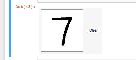
And the prediction of our own handwritten digit is accurate.

Amazon SageMaker notebook – cleanup

After you have finished with this example, remember to delete the prediction endpoint to release the instances associated with it.

estimator.delete_endpoint()

Conclusion

In this blog post we show you how to use the Amazon SageMaker pre-built PyTorch container to build a deep learning model on images, but that’s just the beginning. PyTorch unlocks a huge amount of flexibility, and Amazon SageMaker has provided other example notebooks for image classification on CIFAR-10 and sentiment analysis using recurrent neural networks. We also have TensorFlow example notebooks which you can use to test the latest versions. Or, try it out on your own use case!

About the Author

David Arpin is AWS’s AI Platforms Selection Leader and has a background in managing Data Science teams and Product Management.

Nadia Yakimakha is a Software Development Engineer at AWS working on Machine Learning Frameworks in SageMaker.