AWS Big Data Blog
Extend geospatial queries in Amazon Athena with UDFs and AWS Lambda
Amazon Athena is a serverless and interactive query service that allows you to easily analyze data in Amazon Simple Storage Service (Amazon S3) and 25-plus data sources, including on-premises data sources or other cloud systems using SQL or Python. Athena built-in capabilities include querying for geospatial data; for example, you can count the number of earthquakes in each Californian county. One disadvantage of analyzing at county-level is that it may give you a misleading impression of which parts of California have had the most earthquakes. This is because the counties aren’t equally sized; a county may have had more earthquakes simply because it’s a big county. What if we wanted a hierarchical system that allowed us to zoom in and out to aggregate data over different equally-sized geographic areas?
In this post, we present a solution that uses Uber’s Hexagonal Hierarchical Spatial Index (H3) to divide the globe into equally-sized hexagons. We then use an Athena user-defined function (UDF) to determine which hexagon each historical earthquake occurred in. Because the hexagons are equally-sized, this analysis gives a fair impression of where earthquakes tend to occur.
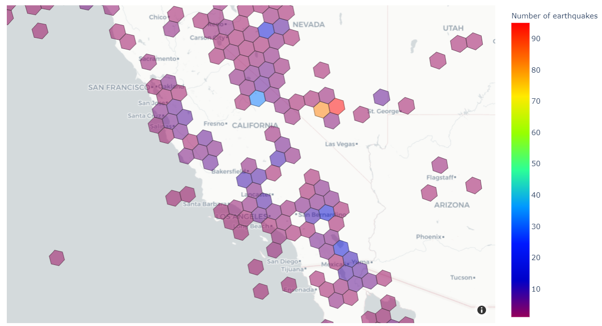
At the end, we’ll produce a visualization like the one below that shows the number of historical earthquakes in different areas of the western US.
H3 divides the globe into equal-sized regular hexagons. The number of hexagons depends on the chosen resolution, which may vary from 0 (122 hexagons, each with edge lengths of about 1,100 km) to 15 (569,707,381,193,162 hexagons, each with edge lengths of about 50 cm). H3 enables analysis at the area level, and each area has the same size and shape.
Solution overview
The solution extends Athena’s built-in geospatial capabilities by creating a UDF powered by AWS Lambda. Finally, we use an Amazon SageMaker notebook to run Athena queries that are rendered as a choropleth map. The following diagram illustrates this architecture.
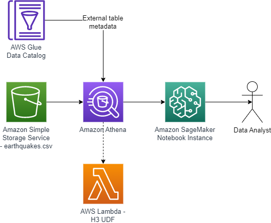
The end-to-end architecture is as follows:
- A CSV file of historical earthquakes is uploaded into an S3 bucket.
- An AWS Glue external table is created based on the earthquake CSV.
- A Lambda function calculates H3 hexagons for parameters (latitude, longitude, resolution). The function is written in Java and can be called as a UDF using queries in Athena.
- A SageMaker notebook uses an AWS SDK for pandas package to run a SQL query in Athena, including the UDF.
- A Plotly Express package renders a choropleth map of the number of earthquakes in each hexagon.
Prerequisites
For this post, we use Athena to read data in Amazon S3 using the table defined in the AWS Glue Data Catalog associated with our earthquake dataset. In terms of permissions, there are two main requirements:
- Athena has access to the S3 bucket where you store the earthquake data and another S3 bucket used to store the output of Athena queries.
- The AWS Identity and Access Management (IAM) role or user you use to run this example is authorized to use Athena. For details, see AWS managed policies for Amazon Athena.
Configure Amazon S3
The first step is to create an S3 bucket to store the earthquake dataset, as follows:
- Download the CSV file of historical earthquakes from GitHub.
- On the Amazon S3 console, choose Buckets in the navigation pane.
- Choose Create bucket.
- For Bucket name, enter a globally unique name for your data bucket.
- Choose Create folder, and enter the folder name
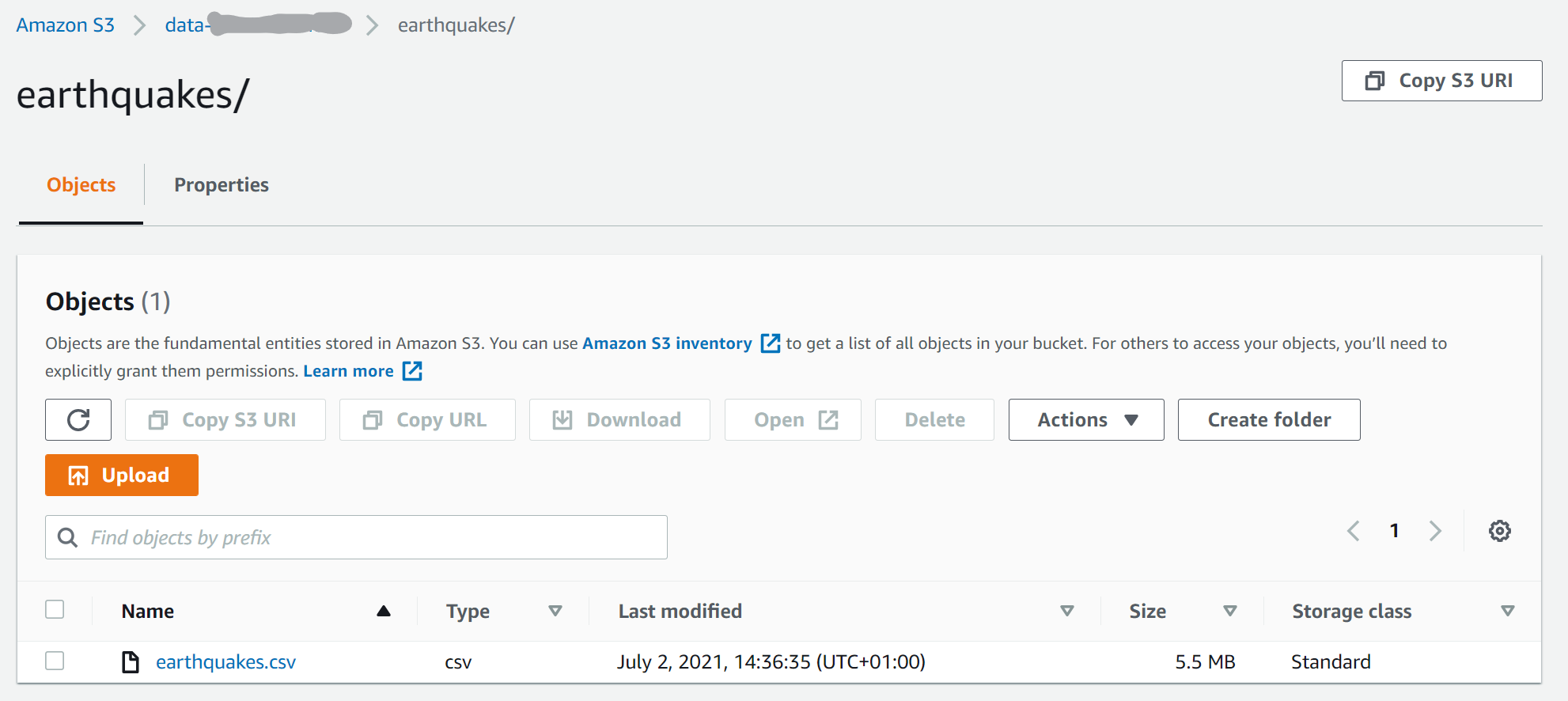
earthquakes. - Upload the file to the S3 bucket. In this example, we upload the
earthquakes.csvfile to theearthquakesprefix.
Create a table in Athena
Navigate to Athena console to create a table. Complete the following steps:
- On the Athena console, choose Query editor.
- Select your preferred Workgroup using the drop-down menu.

- In the SQL editor, use the following code to create a table in the default database:
Create a Lambda function for the Athena UDF
For a thorough explanation on how to build Athena UDFs, see Querying with user defined functions. We use Java 11 and Uber H3 Java binding to build the H3 UDF. We provide the implementation of the UDF on GitHub.
There are several options for deploying a UDF using Lambda. In this example, we use the AWS Management Console. For production deployments, you probably want to use infrastructure as code such as the AWS Cloud Development Kit (AWS CDK). For information about how to use the AWS CDK to deploy the Lambda function, refer to the project code repository. Another possible deployment option is using AWS Serverless Application Repository (SAR).
Deploy the UDF
Deploy the Uber H3 binding UDF using the console as follows:
- Go to binary directory in the GitHub repository, and download
aws-h3-athena-udf-*.jarto your local desktop. - Create a Lambda function called
H3UDFwith Runtime set to Java 11 (Corretto), and Architecture set to x86_64.

- Upload the
aws-h3-athena-udf*.jarfile.

- Change the handler name to
com.aws.athena.udf.h3.H3AthenaHandler.

- In the General configuration section, choose Edit to set the memory of the Lambda function to 4096 MB, which is an amount of memory that works for our examples. You may need to set the memory size larger for your use cases.

Use the Lambda function as an Athena UDF
After you create the Lambda function, you’re ready to use it as a UDF. The following screenshot shows the function details.
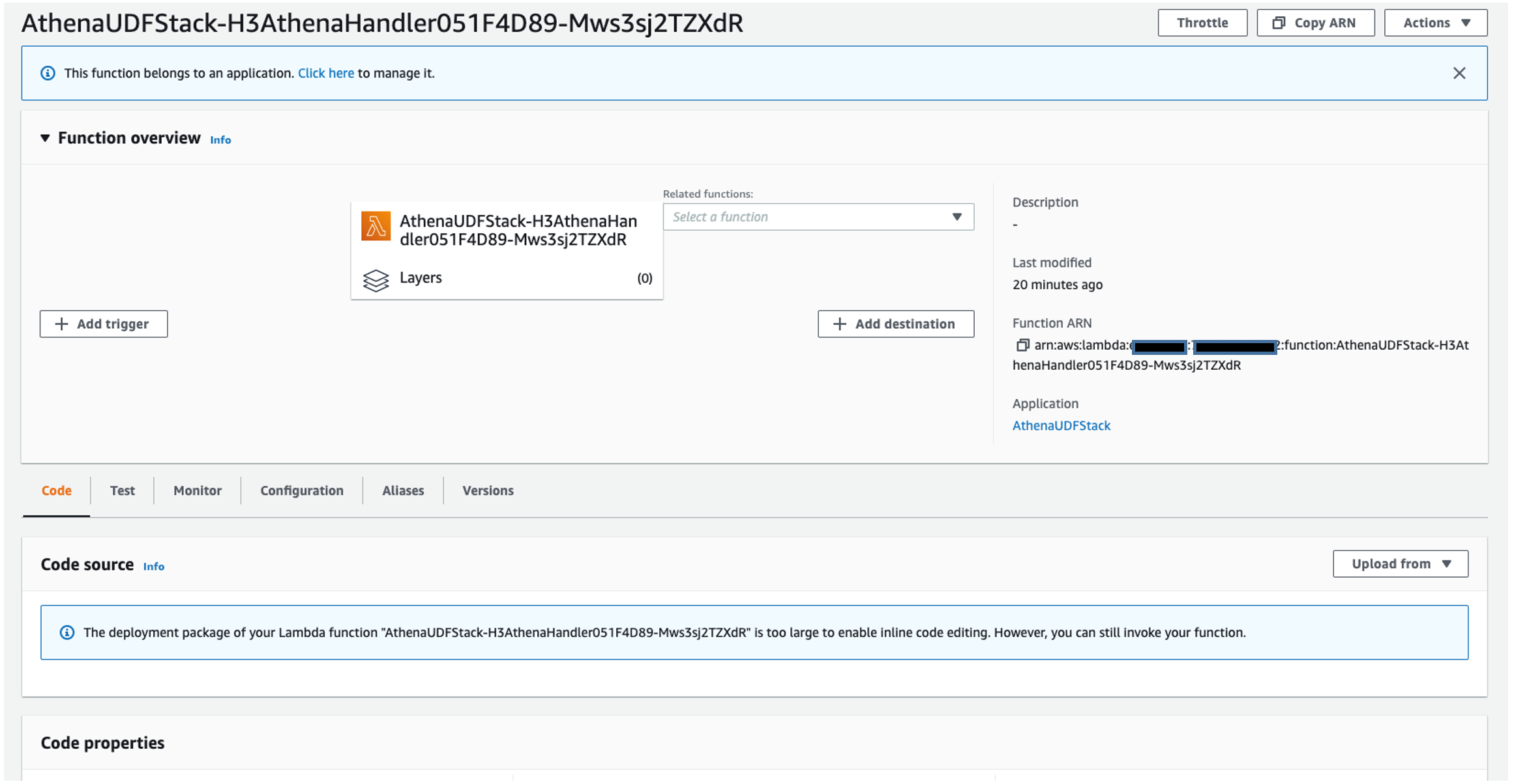
You can now use the function as an Athena UDF. On the Athena console, run the following command:

The udf/examples folder in the GitHub repository includes more examples of the Athena queries.
Developing the UDFs
Now that we showed you how to deploy a UDF for Athena using Lambda, let’s dive deeper into how to develop these kinds of UDFs. As explained in Querying with user defined functions, in order to develop a UDF, we first need to implement a class that inherits UserDefinedFunctionHandler. Then we need to implement the functions inside the class that can be used as UDFs of Athena.
We begin the UDF implementation by defining a class H3AthenaHandler that inherits the UserDefinedFunctionHandler. Then we implement functions that act as wrappers of functions defined in the Uber H3 Java binding. We make sure that all the functions defined in the H3 Java binding API are mapped, so that they can be used in Athena as UDFs. For example, we map the lat_lng_to_cell_address function used in the preceding example to the latLngToCell of the H3 Java binding.
On top of the call to the Java binding, many of the functions in the H3AthenaHandler check whether the input parameter is null. The null check is useful because we don’t assume the input to be non-null. In practice, null values for an H3 index or address are not unusual.
The following code shows the implementation of the get_resolution function:
Some H3 API functions such as cellToLatLng return List<Double> of two elements, where the first element is the latitude and the second is longitude. The H3 UDF that we implement provides a function that returns well-known text (WKT) representation. For example, we provide cell_to_lat_lng_wkt, which returns a Point WKT string instead of List<Double>. We can then use the output of cell_to_lat_lng_wkt in combination with the built-in spatial Athena function ST_GeometryFromText as follows:
Athena UDF only supports scalar data types and does not support nested types. However, some H3 APIs return nested types. For example, the polygonToCells function in H3 takes a List<List<List<GeoCoord>>>. Our implementation of polygon_to_cells UDF receives a Polygon WKT instead. The following shows an example Athena query using this UDF:
Use SageMaker notebooks for visualization
A SageMaker notebook is a managed machine learning compute instance that runs a Jupyter notebook application. In this example, we will use a SageMaker notebook to write and run our code to visualize our results, but if your use case includes Apache Spark then using Amazon Athena for Apache Spark would be a great choice. For advice on security best practices for SageMaker, see Building secure machine learning environments with Amazon SageMaker. You can create your own SageMaker notebook by following these instructions:
- On the SageMaker console, choose Notebook in the navigation pane.
- Choose Notebook instances.
- Choose Create notebook instance.
- Enter a name for the notebook instance.
- Choose an existing IAM role or create a role that allows you to run SageMaker and grants access to Amazon S3 and Athena.
- Choose Create notebook instance.

- Wait for the notebook status to change from
CreatingtoInService. - Open the notebook instance by choosing Jupyter or JupyterLab.
Explore the data
We’re now ready to explore the data.
- On the Jupyter console, under New, choose Notebook.
- On the Select Kernel drop-down menu, choose conda_python3.
- Add new cells by choosing the plus sign.
- In your first cell, download the following Python modules that aren’t included in the standard SageMaker environment:
GeoJSON is a popular format for storing spatial data in a JSON format. The
geojsonmodule allows you to easily read and write GeoJSON data with Python. The second module we install,awswrangler, is the AWS SDK for pandas. This is a very easy way to read data from various AWS data sources into Pandas data frames. We use it to read earthquake data from the Athena table. - Next, we import all the packages that we use to import the data, reshape it, and visualize it:
- We begin importing our data using the
athena.read_sql._queryfunction in AWS SDK for pandas. The Athena query has a subquery that uses the UDF to add a columnh3_cellto each row in theearthquakestable, based on the latitude and longitude of the earthquake. The analytic functionCOUNTis then used to find out the number of earthquakes in each H3 cell. For this visualization, we’re only interested in earthquakes within the US, so we filter out rows in the data frame that are outside the area of interest:The following screenshot shows our results.

Follow along with the rest of the steps in our Jupyter notebook to see how we analyze and visualize our example with H3 UDF data.
Visualize the results
To visualize our results, we use the Plotly Express module to create a choropleth map of our data. A choropleth map is a type of visualization that is shaded based on quantitative values. This is a great visualization for our use case because we’re shading different regions based on the frequency of earthquakes.
In the resulting visual, we can see the ranges of frequency of earthquakes in different areas of North America. Note, the H3 resolution in this map is lower than in the earlier map, which makes each hexagon cover a larger area of the globe.

Clean up
To avoid incurring extra charges on your account, delete the resources you created:
- On the SageMaker console, select the notebook and on the Actions menu, choose Stop.
- Wait for the status of the notebook to change to
Stopped, then select the notebook again and on the Actions menu, choose Delete. - On the Amazon S3 console, select the bucket you created and choose Empty.
- Enter the bucket name and choose Empty.
- Select the bucket again and choose Delete.
- Enter the bucket name and choose Delete bucket.
- On the Lambda console, select the function name and on the Actions menu, choose Delete.
Conclusion
In this post, you saw how to extend functions in Athena for geospatial analysis by adding your own user-defined function. Although we used Uber’s H3 geospatial index in this demonstration, you can bring your own geospatial index for your own custom geospatial analysis.
In this post, we used Athena, Lambda, and SageMaker notebooks to visualize the results of our UDFs in the western US. Code examples are in the h3-udf-for-athena GitHub repo.
As a next step, you can modify the code in this post and customize it for your own needs to gain further insights from your own geographical data. For example, you could visualize other cases such as droughts, flooding, and deforestation.
About the Authors
 John Telford is a Senior Consultant at Amazon Web Services. He is a specialist in big data and data warehouses. John has a Computer Science degree from Brunel University.
 Anwar Rizal is a Senior Machine Learning consultant based in Paris. He works with AWS customers to develop data and AI solutions to sustainably grow their business.
 Pauline Ting is a Data Scientist in the AWS Professional Services team. She supports customers in achieving and accelerating their business outcome by developing sustainable AI/ML solutions. In her spare time, Pauline enjoys traveling, surfing, and trying new dessert places.