AWS Big Data Blog
Extract time series from satellite weather data with AWS Lambda
Extracting time series on given geographical coordinates from satellite or Numerical Weather Prediction data can be challenging because of the volume of data and of its multidimensional nature (time, latitude, longitude, height, multiple parameters). This type of processing can be found in weather and climate research, but also in applications like photovoltaic and wind power. For instance, time series describing the quantity of solar energy reaching specific geographical points can help in designing photovoltaic power plants, monitoring their operation, and detecting yield loss.
A generalization of the problem could be stated as follows: how can we extract data along a dimension that is not the partition key from a large volume of multidimensional data? For tabular data, this problem can be easily solved with AWS Glue, which you can use to create a job to filter and repartition the data, as shown at the end of this post. But what if the data is multidimensional and provided in a domain-specific format, like in the use case that we want to tackle?
AWS Lambda is a serverless compute service that lets you run code without provisioning or managing servers. With AWS Step Functions, you can launch parallel runs of Lambda functions. This post shows how you can use these services to run parallel tasks, with the example of time series extraction from a large volume of satellite weather data stored on Amazon Simple Storage Service (Amazon S3). You also use AWS Glue to consolidate the files produced by the parallel tasks.
Note that Lambda is a general purpose serverless engine. It has not been specifically designed for heavy data transformation tasks. We are using it here after having confirmed the following:
- Task duration is predictable and is less than 15 minutes, which is the maximum timeout for Lambda functions
- The use case is simple, with low compute requirements and no external dependencies that could slow down the process
We work on a dataset provided by EUMESAT: the MSG Total and Diffuse Downward Surface Shortwave Flux (MDSSFTD). This dataset contains satellite data at 15-minute intervals, in netcdf format, which represents approximately 100 GB for 1 year.
We process the year 2018 to extract time series on 100 geographical points.

Solution overview
To achieve our goal, we use parallel Lambda functions. Each Lambda function processes 1 day of data: 96 files representing a volume of approximately 240 MB. We then have 365 files containing the extracted data for each day, and we use AWS Glue to concatenate them for the full year and split them across the 100 geographical points. This workflow is shown in the following architecture diagram.

Deployment of this solution: In this post, we provide step-by-step instructions to deploy each part of the architecture manually. If you prefer an automatic deployment, we have prepared for you a Github repository containing the required infrastructure as code template.
The dataset is partitioned by day, with YYYY/MM/DD/ prefixes. Each partition contains 96 files that will be processed by one Lambda function.
We use Step Functions to launch the parallel processing of the 365 days of the year 2018. Step Functions helps developers use AWS services to build distributed applications, automate processes, orchestrate microservices, and create data and machine learning (ML) pipelines.
But before starting, we need to download the dataset and upload it to an S3 bucket.
Prerequisites
Create an S3 bucket to store the input dataset, the intermediate outputs, and the final outputs of the data extraction.
Download the dataset and upload it to Amazon S3
A free registration on the data provider website is required to download the dataset. To download the dataset, you can use the following command from a Linux terminal. Provide the credentials that you obtained at registration. Your Linux terminal could be on your local machine, but you can also use an AWS Cloud9 instance. Make sure that you have at least 100 GB of free storage to handle the entire dataset.
Because the dataset is quite large, this download could take a long time. In the meantime, you can prepare the next steps.
When the download is complete, you can upload the dataset to an S3 bucket with the following command:
If you use temporary credentials, they might expire before the copy is complete. In this case, you can resume by using the aws s3 sync command.
Now that the data is on Amazon S3, you can delete the directory that has been downloaded from your Linux machine.
Create the Lambda functions
For step-by-step instructions on how to create a Lambda function, refer to Getting started with Lambda.
The first Lambda function in the workflow generates the list of days that we want to process:
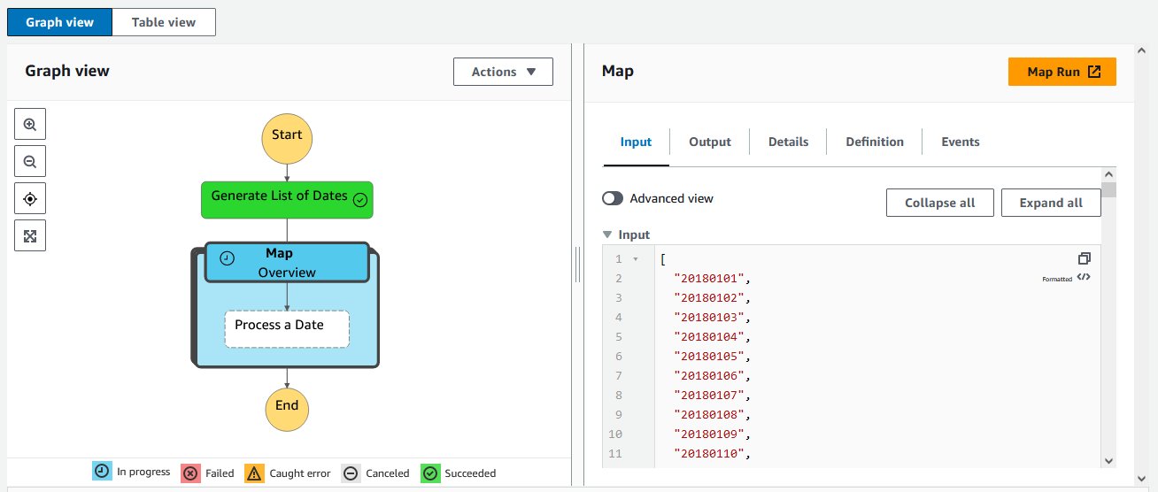
We then use the Map state of Step Functions to process each day. The Map state will launch one Lambda function for each element returned by the previous function, and will pass this element as an input. These Lambda functions will be launched simultaneously for all the elements in the list. The processing time for the full year will therefore be identical to the time needed to process 1 single day, allowing scalability for long time series and large volumes of input data.
The following is an example of code for the Lambda function that processes each day:
You need to associate a role to the Lambda function to authorize it to access the S3 buckets. Because the runtime is about a minute, you also have to configure the timeout of the Lambda function accordingly. Let’s set it to 5 minutes. We also increase the memory allocated to the Lambda function to 2048 MB, which is needed by the netcdf4 library for extracting several points at a time from satellite data.
This Lambda function depends on the pandas and netcdf4 libraries. They can be installed as Lambda layers. The pandas library is provided as an AWS managed layer. The netcdf4 library will have to be packaged in a custom layer.
Configure the Step Functions workflow
After you create the two Lambda functions, you can design the Step Functions workflow in the visual editor by using the Lambda Invoke and Map blocks, as shown in the following diagram.

In the Map state block, choose Distributed processing mode and increase concurrency limit to 365 in Runtime settings. This will enable parallel processing of all the days.


The number of Lambda functions that can run concurrently is limited for each account. Your account may have insufficient quota. You can request a quota increase.
Launch the state machine
You can now launch the state machine. On the Step Functions console, navigate to your state machine and choose Start execution to run your workflow.

This will trigger a popup in which you can enter optional input for your state machine. For this post, you can leave the defaults and choose Start execution.

The state machine should take 1–2 minutes to run, during which time you will be able to monitor the progress of your workflow. You can select one of the blocks in the diagram and inspect its input, output, and other information in real time, as shown in the following screenshot. This can be very useful for debugging purposes.
When all the blocks turn green, the state machine is complete. At this step, we have extracted the data for 100 geographical points for a whole year of satellite data.
In the S3 bucket configured as output for the processing Lambda function, we can check that we have one file per day, containing the data for all the 100 points.

Transform data per day to data per geographical point with AWS Glue
For now, we have one file per day. However, our goal is to get time series for every geographical point. This transformation involves changing the way the data is partitioned. From a day partition, we have to go to a geographical point partition.
Fortunately, this operation can be done very simply with AWS Glue.
- On the AWS Glue Studio console, create a new job and choose Visual with a blank canvas.
For this example, we create a simple job with a source and target block.
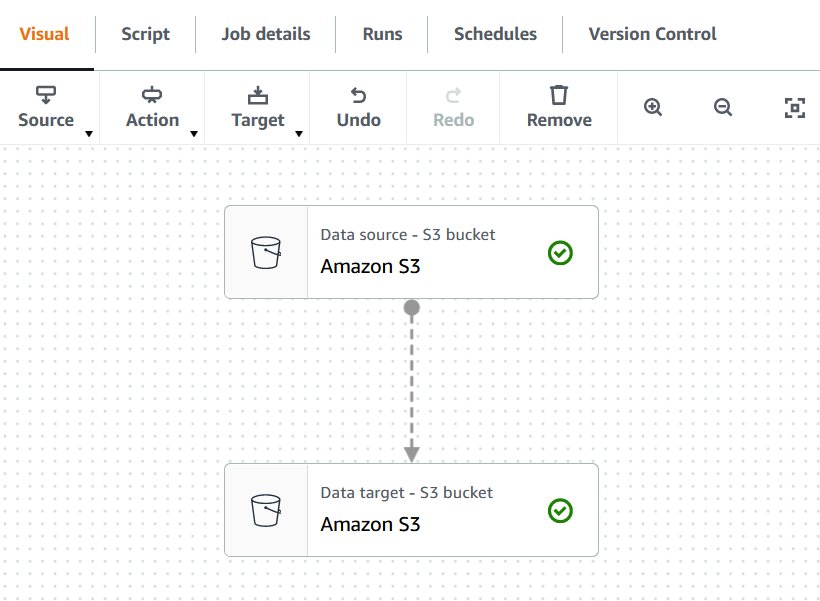
- Add a data source block.
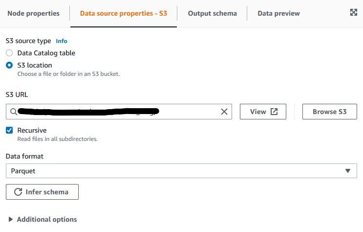
- On the Data source properties tab, select S3 location for S3 source type.
- For S3 URL, enter the location where you created your files in the previous step.
- For Data format, keep the default as Parquet.
- Choose Infer schema and view the Output schema tab to confirm the schema has been correctly detected.
- Add a data target block.
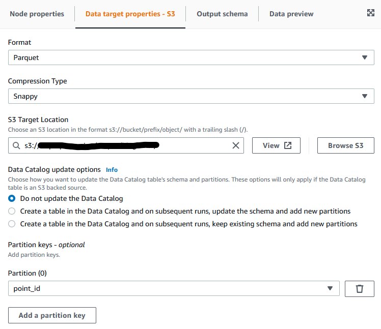
- On the Data target properties tab, for Format, choose Parquet.
- For Compression type, choose Snappy.
- For S3 Target Location, enter the S3 target location for your output files.
We now have to configure the magic!
- Add a partition key, and choose
point_id.
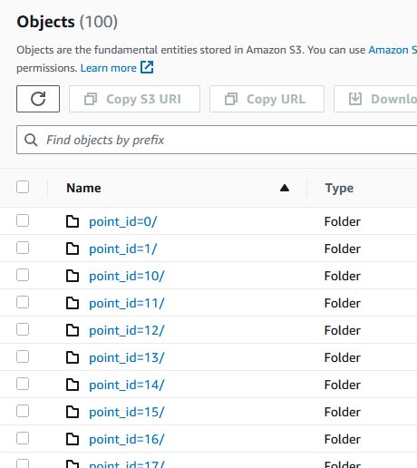
This tells AWS Glue how you want your output data to be partitioned. AWS Glue will automatically partition the output data according to the point_id column, and therefore we’ll get one folder for each geographical point, containing the whole time series for this point as requested.
To finish the configuration, we need to assign an AWS Identity and Access Management (IAM) role to the AWS Glue job.
- Choose Job details, and for IAM role¸ choose a role that has permissions to read from the input S3 bucket and to write to the output S3 bucket.
You may have to create the role on the IAM console if you don’t already have an appropriate one.
- Enter a name for our AWS Glue job, save it, and run it.
We can monitor the run by choosing Run details. It should take 1–2 minutes to complete.
Final results
After the AWS Glue job succeeds, we can check in the output S3 bucket that we have one folder for each geographical point, containing some Parquet files with the whole year of data, as expected.
To load the time series for a specific point into a pandas data frame, you can use the awswrangler library from your Python code:
If you want to test this code now, you can create a notebook instance in Amazon SageMaker, and then open a Jupyter notebook. The following screenshot illustrates running the preceding code in a Jupyter notebook.
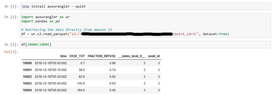
As we can see, we have successfully extracted the time series for specific geographical points!
Clean up
To avoid incurring future charges, delete the resources that you have created:
- The S3 bucket
- The AWS Glue job
- The Step Functions state machine
- The two Lambda functions
- The SageMaker notebook instance
Conclusion
In this post, we showed how to use Lambda, Step Functions, and AWS Glue for serverless ETL (extract, transform, and load) on a large volume of weather data. The proposed architecture enables extraction and repartitioning of the data in just a few minutes. It’s scalable and cost-effective, and can be adapted to other ETL and data processing use cases.
Interested in learning more about the services presented in this post? You can find hands-on labs to improve your knowledge with AWS Workshops. Additionally, check out the official documentation of AWS Glue, Lambda, and Step Functions. You can also discover more architectural patterns and best practices at AWS Whitepapers & Guides.
About the Author

Lior Perez is a Principal Solutions Architect on the Enterprise team based in Toulouse, France. He enjoys supporting customers in their digital transformation journey, using big data and machine learning to help solve their business challenges. He is also personally passionate about robotics and IoT, and constantly looks for new ways to leverage technologies for innovation.