Artificial Intelligence
Announcing the Preview of Amazon SageMaker Profiler: Track and visualize detailed hardware performance data for your model training workloads
Today, we’re pleased to announce the preview of Amazon SageMaker Profiler, a capability of Amazon SageMaker that provides a detailed view into the AWS compute resources provisioned during training deep learning models on SageMaker. With SageMaker Profiler, you can track all activities on CPUs and GPUs, such as CPU and GPU utilizations, kernel runs on GPUs, kernel launches on CPUs, sync operations, memory operations across GPUs, latencies between kernel launches and corresponding runs, and data transfer between CPUs and GPUs. In this post, we walk you through the capabilities of SageMaker Profiler.
SageMaker Profiler provides Python modules for annotating PyTorch or TensorFlow training scripts and activating SageMaker Profiler. It also offers a user interface (UI) that visualizes the profile, a statistical summary of profiled events, and the timeline of a training job for tracking and understanding the time relationship of the events between GPUs and CPUs.
The need for profiling training jobs
With the rise of deep learning (DL), machine learning (ML) has become compute and data intensive, typically requiring multi-node, multi-GPU clusters. As state-of-the-art models grow in size in the order of trillions of parameters, their computational complexity and cost also increase rapidly. ML practitioners have to cope with common challenges of efficient resource utilization when training such large models. This is particularly evident in large language models (LLMs), which typically have billions of parameters and therefore require large multi-node GPU clusters in order to train them efficiently.
When training these models on large compute clusters, we can encounter compute resource optimization challenges such as I/O bottlenecks, kernel launch latencies, memory limits, and low resource utilizations. If the training job configuration is not optimized, these challenges can result in inefficient hardware utilization and longer training times or incomplete training runs, which increase the overall costs and timelines for the project.
Prerequisites
The following are the prerequisites to start using SageMaker Profiler:
- A SageMaker domain in your AWS account – For instructions on setting up a domain, see Onboard to Amazon SageMaker Domain using quick setup. You also need to add domain user profiles for individual users to access the SageMaker Profiler UI application. For more information, see Add and remove SageMaker Domain user profiles.
- Permissions – The following list is the minimum set of permissions that should be assigned to the execution role for using the SageMaker Profiler UI application:
sagemaker:CreateAppsagemaker:DeleteAppsagemaker:DescribeTrainingJobsagemaker:SearchTrainingJobss3:GetObjects3:ListBucket
Prepare and run a training job with SageMaker Profiler
To start capturing kernel runs on GPUs while the training job is running, modify your training script using the SageMaker Profiler Python modules. Import the library and add the start_profiling() and stop_profiling() methods to define the beginning and the end of profiling. You can also use optional custom annotations to add markers in the training script to visualize hardware activities during particular operations in each step.
There are two approaches that you can take to profile your training scripts with SageMaker Profiler. The first approach is based on profiling full functions; the second approach is based on profiling specific code lines in functions.
To profile by functions, use the context manager smppy.annotate to annotate full functions. The following example script shows how to implement the context manager to wrap the training loop and full functions in each iteration:
You can also use smppy.annotation_begin() and smppy.annotation_end() to annotate specific lines of code in functions. For more information, refer to documentation.
Configure the SageMaker training job launcher
After you’re done annotating and setting up the profiler initiation modules, save the training script and prepare the SageMaker framework estimator for training using the SageMaker Python SDK.
- Set up a
profiler_configobject using theProfilerConfigandProfilermodules as follows: - Create a SageMaker estimator with the
profiler_configobject created in the previous step. The following code shows an example of creating a PyTorch estimator:
If you want to create a TensorFlow estimator, import sagemaker.tensorflow.TensorFlow instead, and specify one of the TensorFlow versions supported by SageMaker Profiler. For more information about supported frameworks and instance types, see Supported frameworks.
- Start the training job by running the fit method:
Launch the SageMaker Profiler UI
When the training job is complete, you can launch the SageMaker Profiler UI to visualize and explore the profile of the training job. You can access the SageMaker Profiler UI application through the SageMaker Profiler landing page on the SageMaker console or through the SageMaker domain.
To launch the SageMaker Profiler UI application on the SageMaker console, complete the following steps:
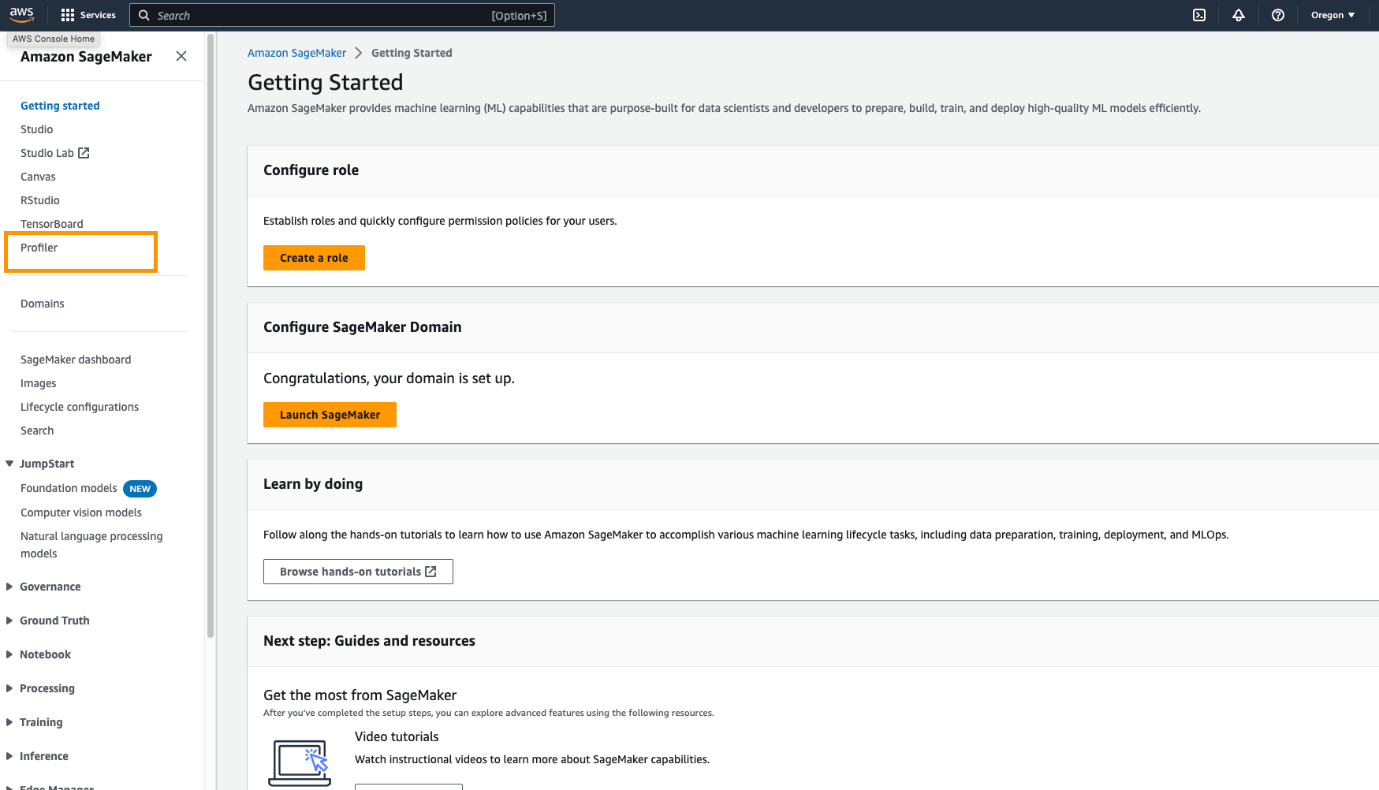
- On the SageMaker console, choose Profiler in the navigation pane.
- Under Get started, select the domain in which you want to launch the SageMaker Profiler UI application.
If your user profile only belongs to one domain, you will not see the option for selecting a domain.
- Select the user profile for which you want to launch the SageMaker Profiler UI application.
If there is no user profile in the domain, choose Create user profile. For more information about creating a new user profile, see Add and Remove User Profiles.
- Choose Open Profiler.
You can also launch the SageMaker Profiler UI from the domain details page.
Gain insights from the SageMaker Profiler
When you open the SageMaker Profiler UI, the Select and load a profile page opens, as shown in the following screenshot.
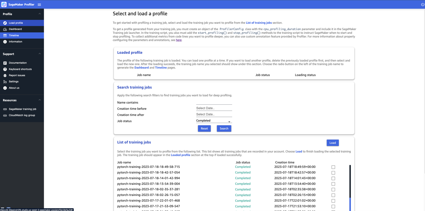
You can view a list of all the training jobs that have been submitted to SageMaker Profiler and search for a particular training job by its name, creation time, and run status (In Progress, Completed, Failed, Stopped, or Stopping). To load a profile, select the training job you want to view and choose Load. The job name should appear in the Loaded profile section at the top.
Choose the job name to generate the dashboard and timeline. Note that when you choose the job, the UI automatically opens the dashboard. You can load and visualize one profile at a time. To load another profile, you must first unload the previously loaded profile. To unload a profile, choose the trash bin icon in the Loaded profile section.
For this post, we view the profile of an ALBEF training job on two ml.p4d.24xlarge instances.
After you finish loading and selecting the training job, the UI opens the Dashboard page, as shown in the following screenshot.
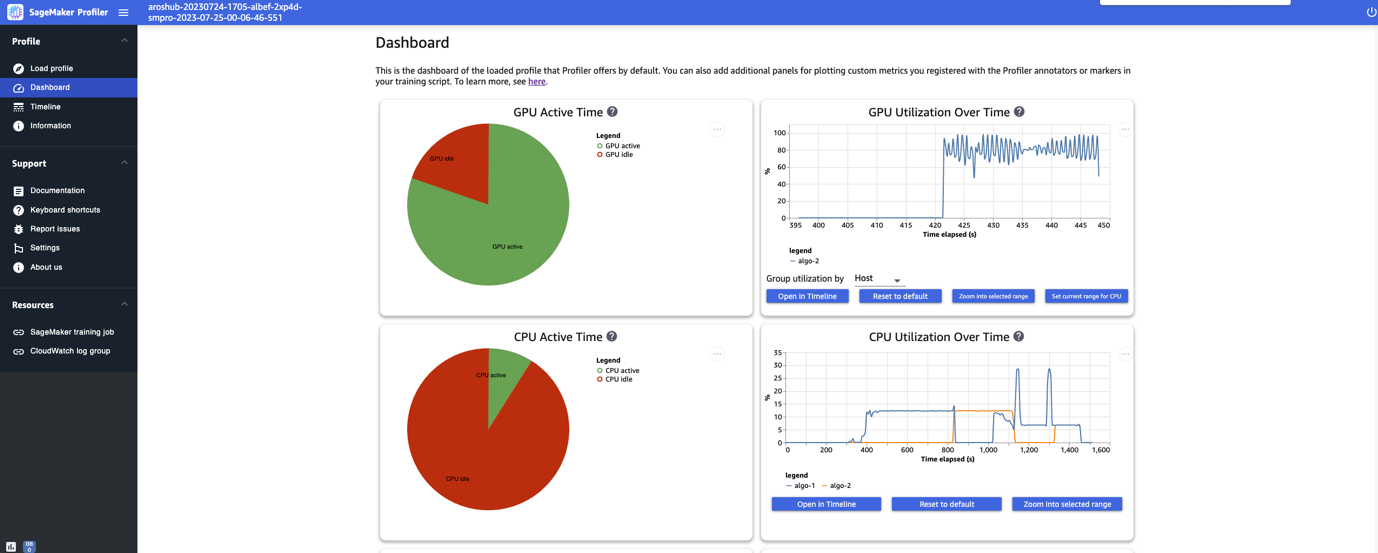
You can see the plots for key metrics, namely the GPU active time, GPU utilization over time, CPU active time, and CPU utilization over time. The GPU active time pie chart shows the percentage of GPU active time vs. GPU idle time, which enables us to check if the GPUs are more active than idle throughout the entire training job. The GPU utilization over time timeline graph shows the average GPU utilization rate over time per node, aggregating all the nodes in a single chart. You can check if the GPUs have an unbalanced workload, under-utilization issues, bottlenecks, or idle issues during certain time intervals. For more details on interpreting these metrics, refer to documentation.
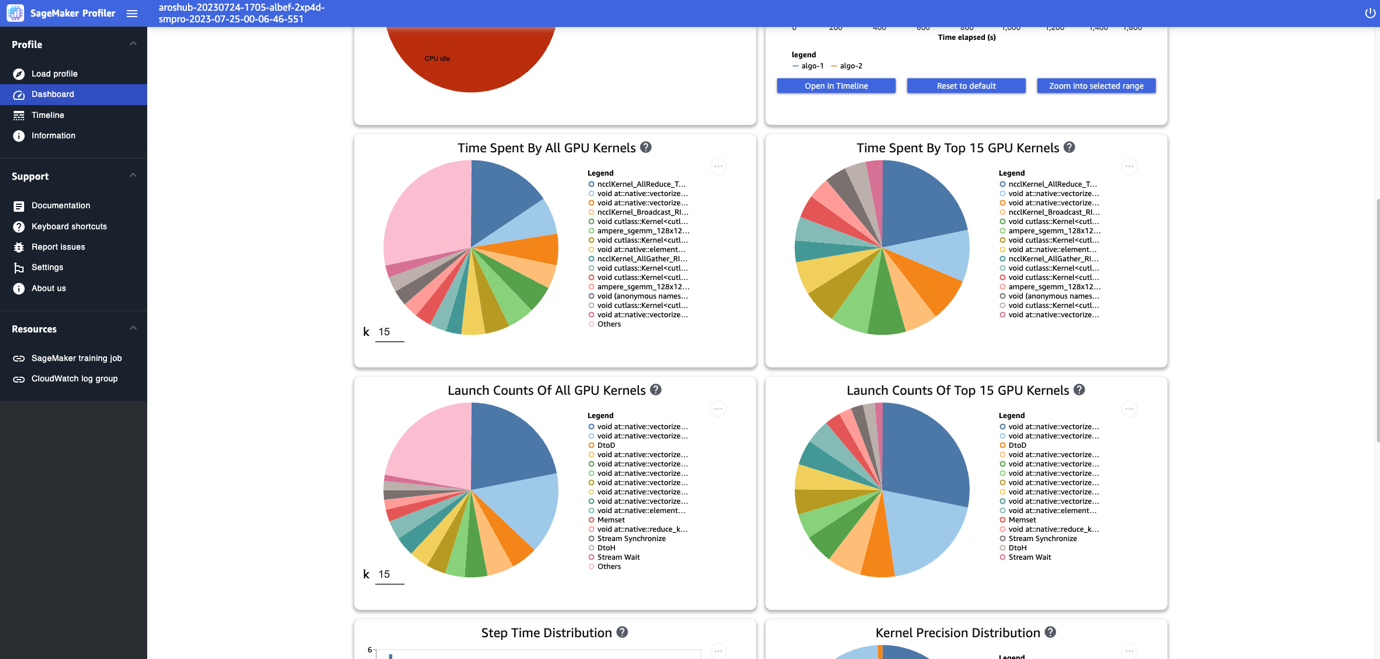
The dashboard provides you with additional plots, including time spent by all GPU kernels, time spent by the top 15 GPU kernels, launch counts of all GPU kernels, and launch counts of the top 15 GPU kernels, as shown in the following screenshot.
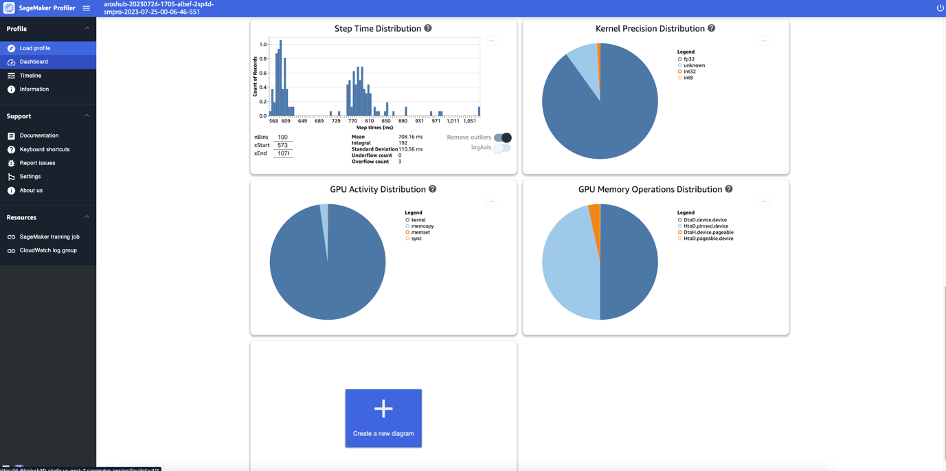
Lastly, the dashboard enables you to visualize additional metrics, such as the step time distribution, which is a histogram that shows the distribution of step durations on GPUs, and the kernel precision distribution pie chart, which shows the percentage of time spent on running kernels in different data types such as FP32, FP16, INT32, and INT8.
You can also obtain a pie chart on the GPU activity distribution that shows the percentage of time spent on GPU activities, such as running kernels, memory (memcpy and memset), and synchronization (sync). You can visualize the percentage of time spent on GPU memory operations from the GPU memory operations distribution pie chart.
You can also create your own histograms based on a custom metric that you annotated manually as described earlier in this post. When adding a custom annotation to a new histogram, select or enter the name of the annotation you added in the training script.
Timeline interface
The SageMaker Profiler UI also includes a timeline interface, which provides you with a detailed view into the compute resources at the level of operations and kernels scheduled on the CPUs and run on the GPUs. The timeline is organized in a tree structure, giving you information from the host level to the device level, as shown in the following screenshot.
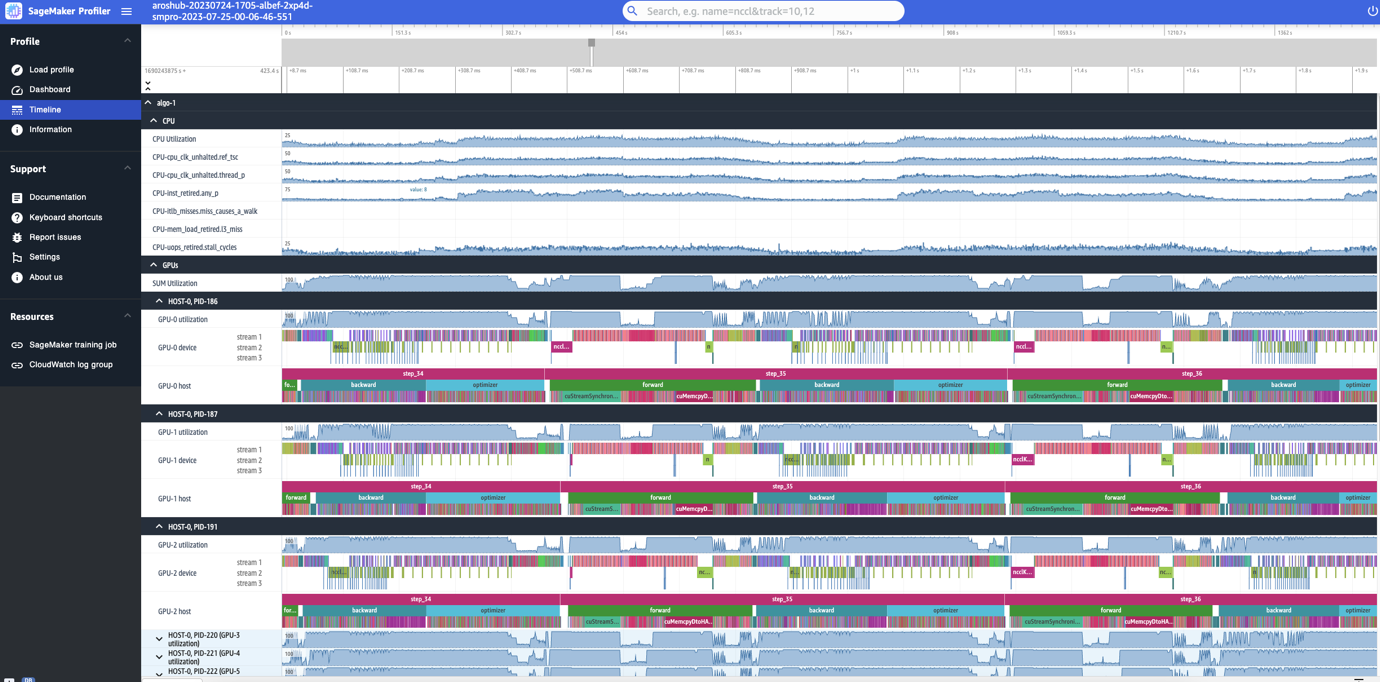
For each CPU, you can track the CPU performance counters, such as clk_unhalted_ref.tsc and itlb_misses.miss_causes_a_walk. For each GPU on the 2x p4d.24xlarge instance, you can see a host timeline and a device timeline. Kernel launches are on the host timeline and kernel runs are on the device timeline.
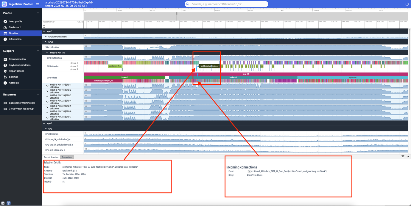
You can also zoom in to the individual steps. In the following screenshot, we have zoomed in to step_41. The timeline strip selected in the following screenshot is the AllReduce operation, an essential communication and synchronization step in distributed training, run on GPU-0. In the screenshot, note that the kernel launch in the GPU-0 host connects to the kernel run in the GPU-0 device stream 1, indicated with the arrow in cyan.
Availability and considerations
SageMaker Profiler is available in PyTorch (version 2.0.0 and 1.13.1) and TensorFlow (version 2.12.0 and 2.11.1). The following table provides the links to the supported AWS Deep Learning Containers for SageMaker.
| Framework | Version | AWS DLC Image URI |
| PyTorch | 2.0.0 | 763104351884.dkr.ecr.<region>.amazonaws.com/pytorch-training:2.0.0-gpu-py310-cu118-ubuntu20.04-sagemaker |
| PyTorch | 1.13.1 | 763104351884.dkr.ecr.<region>.amazonaws.com/pytorch-training:1.13.1-gpu-py39-cu117-ubuntu20.04-sagemaker |
| TensorFlow | 2.12.0 | 763104351884.dkr.ecr.<region>.amazonaws.com/tensorflow-training:2.12.0-gpu-py310-cu118-ubuntu20.04-sagemaker |
| TensorFlow | 2.11.1 | 763104351884.dkr.ecr.<region>.amazonaws.com/tensorflow-training:2.11.1-gpu-py39-cu112-ubuntu20.04-sagemaker |
SageMaker Profiler is currently available in the following Regions: US East (Ohio, N. Virginia), US West (Oregon), and Europe (Frankfurt, Ireland).
SageMaker Profiler is available in the training instance types ml.p4d.24xlarge, ml.p3dn.24xlarge, and ml.g4dn.12xlarge.
For the full list of supported frameworks and versions, refer to documentation.
SageMaker Profiler incurs charges after the SageMaker Free Tier or the free trial period of the feature ends. For more information, see Amazon SageMaker Pricing.
Performance of SageMaker Profiler
We compared the overhead of SageMaker Profiler against various open-source profilers. The baseline used for the comparison was obtained from running the training job without a profiler.
Our key finding revealed that SageMaker Profiler generally resulted in a shorter billable training duration because it had less overhead time on the end-to-end training runs. It also generated less profiling data (up to 10 times less) when compared against open-source alternatives. The smaller profiling artifacts generated by SageMaker Profiler require less storage, thereby also saving on costs.
Conclusion
SageMaker Profiler enables you to get detailed insights into the utilization of compute resources when training your deep learning models. This can enable you to resolve performance hotspots and bottlenecks to ensure efficient resource utilization that would ultimately drive down training costs and reduce the overall training duration.
To get started with SageMaker Profiler, refer to documentation.
About the Authors
 Roy Allela is a Senior AI/ML Specialist Solutions Architect at AWS based in Munich, Germany. Roy helps AWS customers—from small startups to large enterprises—train and deploy large language models efficiently on AWS. Roy is passionate about computational optimization problems and improving the performance of AI workloads.
 Sushant Moon is a Data Scientist at AWS, India, specializing in guiding customers through their AI/ML endeavors. With a diverse background spanning retail, finance, and insurance domains, he delivers innovative and tailored solutions. Beyond his professional life, Sushant finds rejuvenation in swimming and seeks inspiration from his travels to diverse locales.
 Diksha Sharma is an AI/ML Specialist Solutions Architect in the Worldwide Specialist Organization. She works with public sector customers to help them architect efficient, secure, and scalable machine learning applications including generative AI solutions on AWS. In her spare time, Diksha loves to read, paint, and spend time with her family.