AWS Quantum Technologies Blog
Running quantum chemistry calculations using AWS ParallelCluster
 Chris Downing, Senior HPC Consultant, AWS Professional Services
Introduction
Modern computational chemistry drives innovation in areas ranging from drug discovery to material design. One of the most popular electronic structure modelling techniques in computational chemistry is known as Density Functional Theory (DFT). The popularity of DFT is primarily due to the fact that it is computationally more efficient than other traditional techniques in computational chemistry and allows one to achieve a reasonable accuracy for many practically interesting chemical systems.
The key strength of DFT and related electronic structure methods is their ability to provide insights into chemical bonding and reactions – topics which can only be approached via approximations if using empirical methods such as molecular dynamics or other coarse-grained simulations. The challenge posed by electronic structure calculations is one of cost – simulation times typically scale with N3 or worse, where N is the number of electrons in the system. Additionally, most established computational chemistry packages require a high degree of communication between cores when executed in parallel, making efficient execution challenging.
Quantum computing is expected to eventually offer a performance advantage over classical computation for quantum chemistry applications. While current quantum computers are not capable of delivering a speed-up, many research efforts have begun with the aim of developing new algorithms which make use of quantum computing principles, to replace the most computationally expensive classical techniques.
Researchers attempting to benchmark quantum computing or hybrid quantum-classical algorithms desire a baseline result to compare against, necessitating the use of standardized and widely-available scientific software which can already address a variety of accuracy and performance targets. In order to address real industrially-relevant use-cases, these baselines will require the use of multi-node parallelism and other compute resources more commonly associated with high performance computing (HPC).
This blog post is an introduction to HPC on AWS for quantum computing researchers who are seeking to compare their quantum or hybrid algorithms against classical calculations.
We describe the process of deploying an HPC cluster on AWS for computational chemistry calculations, and an example of how to install and run the popular electronic structure theory application QuantumESPRESSO.
Deploying an HPC Environment
The quickest way to get started deploying a HPC environment on AWS is using AWS ParallelCluster. The ParallelCluster command-line tool can be used to deploy a suitable VPC and subnet for creating a HPC cluster, or you can create your own networking components in advance via other tools which are not HPC-specific, such as the AWS Cloud Development Kit (CDK) or CloudFormation.
Cluster installation tools
You can install the ParallelCluster CLI using the Python package installer pip. Tooling is available in Python which allows for the installation of different ParallelCluster versions if necessary, or simply for separating ParallelCluster dependencies from other packages which might be installed locally – some examples to consider are the use of virtual environments or pipx. If not already available in your environment, you should also install the AWS CLI at this time, and configure a set of credentials for accessing your account. Your account administrator can define an appropriate IAM role for use with ParallelCluster by referring to the ParallelCluster documentation.
Before deploying a cluster, we recommend creating a new Amazon S3 bucket which will be used to host the post-install configuration file:
aws s3 mb s3://<your-bucket-name>By default, the aws and pcluster CLIs will use the region specified during the initial AWS CLI configuration – but you can select a different region if desired by adding the --region <region-name> argument to any of the commands described here.
Once ParallelCluster is installed, you can generate a basic configuration file (and deploy networking requirements automatically) using pcluster configure --config cluster.yaml. Note that the file cluster.yaml does not need to exist before running the command – it’s automatically populated during the configuration process.
The pcluster configure process will walk through a series of questions to allow your cluster and VPC to be tailored to your use-case, and checks that certain dependencies – like the presence of an SSH key -are met.
For the purposes of this post, we’ll be making manual edits to the cluster.yaml file after configuration is complete, so you can accept default selections for most of the prompts – if you want to make use of an automatic VPC created by ParallelCluster, just respond “yes” when prompted Automate VPC creation? (y/n). Alternatively, you can use an additional tool like AWS CDK to deploy the networking components.
With the ParallelCluster interactive configuration completed, a VPC (with standard subnets and security groups) will be deployed to your account and a basic configuration file added to your working directory. You can now modify the cluster.yaml file to better suit the needs of your specific application.
The template below is an example which is suitable for running quantum chemistry calculations. Simply replace any networking-related <variables> highlighted with the values from your auto-generated cluster.yaml file, and S3-related variables with references to the bucket described previously, along with any prefix (analogous to a folder) you wish to use when organizing your files:
Image:
  Os: rhel8
HeadNode:
  InstanceType: c5.large
  LocalStorage:
    RootVolume:
      Size: 200
      VolumeType: gp3
      Encrypted: true
  Networking:
    SubnetId: <head-node-subnet>
  Ssh:
    KeyName: <key-name>
  Dcv:
    Enabled: false
  Imds:
    Secured: true
  Iam:
    S3Access:
      - BucketName: <your-config-bucket>
        KeyName: <your-key-prefix>/*
        EnableWriteAccess: false
  CustomActions:
    OnNodeConfigured:
      Script: s3://<your-config-bucket>/<your-key-prefix>/<script-name>
Scheduling:
  Scheduler: slurm
  SlurmQueues:
    - Name: compute
      CapacityType: ONDEMAND
      ComputeSettings:
        LocalStorage:
          RootVolume:
            Size: 50
            VolumeType: gp3
      ComputeResources:
        - Name: c6i32xl
          InstanceType: c6i.32xlarge
          MinCount: 0
          MaxCount: 16
          DisableSimultaneousMultithreading: true
          Efa:
            Enabled: true
      Networking:
        SubnetIds:
          - <compute-node-subnet>
        PlacementGroup:
          Enabled: true
    - Name: highmem
      CapacityType: ONDEMAND
      ComputeSettings:
        LocalStorage:
          RootVolume:
            Size: 50
            VolumeType: gp3
      ComputeResources:
        - Name: i3en24xl
          InstanceType: i3en.24xlarge
          MinCount: 0
          MaxCount: 16
          DisableSimultaneousMultithreading: true
          Efa:
            Enabled: true
      Networking:
        SubnetIds:
          - <compute-node-subnet>
        PlacementGroup:
          Enabled: true
SharedStorage:
  - Name: fsx
    StorageType: FsxLustre
    MountDir: /fsx
    FsxLustreSettings:
      StorageCapacity: 1200
Compute queues in the cluster
If you’re using the instance selection from this template, the cluster is configured with two queues, each accommodating a different instance type, targeted at specific workload characteristics:
- c6i.32xlarge: a compute-optimized instance from the latest generation of x86_64 architecture instances, based on Intel Icelake processors. A good instance type selection for a wide variety of HPC applications, with a balanced memory-per-core ratio of 4 GB per core (when considering physical cores, i.e. with hyperthreading disabled as is common practice for HPC systems). This instance type also benefits from access to AWS Elastic Fabric Adapter (EFA) and 50GB/s network bandwidth.
- i3en.24xlarge: an alternative instance type suited for workloads which require increased memory capacity (16 GB per CPU core) and also benefit from fast local SSDs, which are configured as a single RAID-0 “scratch” space when deployed by ParallelCluster. This instance type includes EFA support and 100GB/s network bandwidth.
Storage considerations
In this post, we’re focusing on the use of the DFT application Quantum ESPRESSO. Since this application does not make heavy use of local “scratch” disk space, we can focus exclusively on c6i.32xlarge compute nodes; but i3en.24xlarge is included in our example to show how the cluster template can be expanded if other compute configurations are required. Since MinCount is set to 0, this queue will stay dormant (and thus won’t cost you anything) unless you send jobs to it.
When running calculations, the primary working space should be the high-performance FSx for Lustre file-system, mounted at /fsx as we specified in the cluster config file. Lustre is a network file-system with clients automatically installed on all nodes as part of the standard ParallelCluster deployment process, so files saved under /fsx will be available on all nodes of the cluster simultaneously. It’s extremely fast, and can be tuned to accommodate almost any I/O requirement.
EBS is the default storage service associated with Amazon EC2 – every instance launched in this example will have an associated EBS volume which serves as storage capacity for the operating system. You can attach additional EBS volumes to the cluster controller instance if you need to by adding an appropriate section to the ParallelCluster configuration file. In this case, we create a larger EBS root volume for the controller (this is where numerical libraries will be installed) and smaller EBS root volumes for each compute node, but we do not add an extra EBS volume as shared storage because that role is being served by the Lustre file-system.
Customizing the software stack
To allow a post-install configuration script to be downloaded and executed as part of the cluster setup, we’ve enabled read-only S3 access for the cluster controller instance (not the compute instances), granting access to the specified bucket/prefix. Multiple bucket/prefix combinations can be specified with different write-access permissions if desired – for example, to allow job output files to be copied to S3 for archiving.
By default, ParallelCluster provides a lightweight software stack suited to building and running simple HPC applications. The key components provided are the OpenMPI and Intel MPI libraries. Both are built with support for libfabric and therefore able to make full use of AWS Elastic Fabric Adapter (EFA).
In this case, we wish to use the latest version of Intel MPI as well as Intel MKL – a highly optimized library of numerical methods. The ParallelCluster configuration file above references a post-install script, which is provided below. The post-install script will be automatically downloaded and executed by any node of the cluster when they first boot if the corresponding section of the config file (CustomActions / OnNodeConfigured) are set.
The file should be uploaded to the location within Amazon S3 specified in the configuration file (i.e., s3://<your-config-bucket>/<your-key-prefix>/<script-name>) using the AWS CLI or the web console.
#!/bin/bash
set -euxo pipefail
exec > >(tee /var/log/post-install.log|logger -t post-install -s 2>/dev/console) 2>&1

install_oneapi(){
cat << 'EOF' > /etc/yum.repos.d/oneAPI.repo
[oneAPI]
name=Intel(R) oneAPI repository
baseurl=https://yum.repos.intel.com/oneapi
enabled=1
gpgcheck=0
repo_gpgcheck=0
gpgkey=https://yum.repos.intel.com/intel-gpg-keys/GPG-PUB-KEY-INTEL-SW-PRODUCTS.PUB
EOF
yum install -y intel-basekit
yum install -y intel-hpckit
}

install_oneapi
The post-install script ensures that the required libraries are installed on the controller node, and since by default ParallelCluster exports the /opt/intel directory to compute nodes via NFS, there is no need to perform any post-install step on the compute nodes themselves. As such, we specify in our cluster config that the post-install step is required for the head node, but not for any of the compute partitions. Avoiding compute-node post-install steps helps to reduce the time between job submission and job runtime, and consequently also reduces the cost of each job.
Once the cluster configuration file is completely populated and the post-install script has been uploaded to S3, the cluster can be deployed by running the command (from the directory where the cluster.yaml file is present):
pcluster create-cluster --cluster-name <your-cluster-name> --cluster-configuration cluster.yamlInstalling QuantumESPRESSO
Once the cluster creation process finishes, you can move on to the installation of QuantumESPRESSO. The latest versions of the software can make use of GPUs and have compatibility with a range of numerical libraries, but for now we will focus on running jobs on Intel CPUs and making use of the OneAPI libraries. The core components (updated versions of Intel MPI and MKL) were installed to the cluster controller node as part of the post-install process shown previously, making compilation of QuantumESPRESSO relatively straightforward.
Begin by checking that the cluster deployment is completed:
pcluster list-clustersOnce the response includes CREATE_COMPLETE for the cluster you are deploying, you can connect to the cluster via SSH:
pcluster ssh --cluster-name <your-cluster-name>Once connected to the cluster, you can proceed with downloading and installing the QuantumESPRESSO package by running the following commands from the SSH session (or by creating a script based on these commands to automate the process):
mkdir -p /fsx/applications/quantum-espresso
cd /fsx/applications/quantum-espresso
wget https://gitlab.com/QEF/q-e/-/archive/qe-7.1/q-e-qe-7.1.tar.gz
tar -xvzf q-e-qe-7.1.tar.gz
cd q-e-qe-7.1
source /opt/intel/oneapi/setvars.sh
./configure
make all
Additional tuning may be possible (e.g., including the ELPA library, or enabling GPU acceleration) for users who are more experienced with software compilation. As an alternative to building the application and its dependencies directly, you can also consider making use of the Spack package manager. For a walk-through of how to deploy Spack on AWS ParallelCluster, please refer to a previous post here on the HPC blog channel.
Running a QuantumESPRESSO Job
Now that you have a cluster with QuantumESPRESSO and its dependencies installed, we can run a test job.
The first step is to prepare inputs for QuantumESPRESSO – namely the batch job script (which will be interpreted by the scheduler, enabling the job to run on a dynamically-created set of compute resources), the QuantumESPRESSO input file, and the collection of pseudopotential files for the elements included in our simulation.
Pseudopotential files which are compatible with QuantumESPRESSO can be downloaded from Materials Cloud. You will need to acknowledge the license disclaimer and download to your local device, upload the bundle of pseudopotential files to S3, then finally download onto your cluster:
Local machine: aws s3 cp SSSP_1.1.2_PBE_efficiency.tar.gz s3://<your-bucket-name>/<your-key-prefix>/
Cluster: aws s3 cp s3://<your-bucket-name>/<your-key-prefix>/SSSP_1.1.2_PBE_efficiency.tar.gz .
Alternatively, copy files directly to the cluster head node using scp:
pcluster describe-cluster --cluster-name <your-cluster-name>(Look for the public IP address for your cluster head node in the JSON output):
scp SSSP_1.1.2_PBE_efficiency.tar.gz ec2-user@<your-public-ip>:~Once the pseudopotential files are uploaded to the cluster head node, reconnect via SSH and create a location within the /fsx mount point for them to reside, and unpack the bundle:
mkdir -p /fsx/resources/pseudopotentials
mv SSSP_1.1.2_PBE_efficiency.tar.gz /fsx/resources/pseudopotentials
cd /fsx/resources/pseudopotentials
tar -xvzf SSSP_1.1.2_PBE_efficiency.tar.gz
With the requirements in place, we can create the QuantumESPRESSO input file. You can use other capabilities of Materials Cloud to choose a crystal structure and use it to generate an input file. To use these tools, locate the crystal structure you wish to investigate and download a structure file (e.g., CIF file), then upload the structure to the input generator and select your desired run-time parameters.
For this demonstration, we can envisage a researcher developing quantum computing and hybrid algorithms which can target the calculation of formation energies for defects in a crystal structure. Since the formation energy for a defect is relative to the pure/unmodified structure, the first step would be to calculate the internal energy of a pure material. Here we’ll use the “Pmmm” space-group crystal structure of Ta2O5 as an example, using a “very fine” k-point mesh and fractional occupations.
Once you’ve obtained a QuantumESPRESSO input file by following the steps described above, copy the contents to a file on the cluster (e.g. Ta2O5.in), located in a directory which will be accessible to the compute nodes as well as the head node – this could either be your /home directory, or a directory within the /fsx mount point.
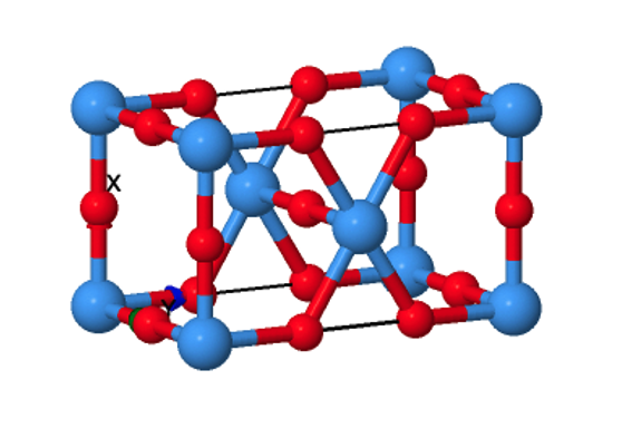
Figure 1: Pmmm space group structure of Ta2O5. While most simple metal oxides have crystal structures which have been conclusively determined for decades, definitive structures for Ta2O5 have proved more difficult to isolate experimentally.
Update the Ta2O5.in file (or your custom equivalent) so that the pseudo_dir option points to the location where your pseudopotential files are saved (e.g. pseudo_dir = '/fsx/resources/pseudopotentials'), and ensure that the correct pseudopotential files are specified in your input file by comparing the filenames listed under the ATOMIC_SPECIES directive against the directory contents.
The input file we have created so far is sufficient to run a standard DFT calculation, but to fully showcase the performance and scalability of the compute environment we have created, we will use the higher order method “hybrid DFT”. This approach incorporates a fraction of the exact exchange term calculated using Hartree-Fock theory, and so in principle offers higher accuracy with the trade-off of greater computational cost.
To configure the job to run a hybrid DFT calculation, simply add the following lines to the &SYSTEM directive in the input file:
input_dft='pbe0'
nqx1=1
nqx2=1
nqx3=1
With the QuantumESPRESSO input files complete, you can move on to preparing a Slurm batch submission script. The key parameters to set within the job script are the number of cores and/or number of nodes desired, as well as the partition to be used. In this example, each partition contains only a single compute node type, though ParallelCluster supports multiple instance types within the same partition and a larger number of separate partitions than we have specified here.
Since we are using c6i.32xlarge instances as our primary compute nodes and have disabled multi-threading in the cluster configuration file, we know that each node will have 64 CPU cores. Our jobs should therefore be sized to use a multiple of this value in order to maximally utilize each of the nodes we launch.
Below is an example job script, demonstrating how to set up a job to run via the Slurm scheduler:
#!/bin/bash
#SBATCH -J Ta2O5
#SBATCH -N 2
#SBATCH -n 128
#SBATCH --partition=compute
#SBATCH --exclusive

module purge
source /opt/intel/oneapi/setvars.sh --force

QEBIN=/fsx/applications/quantum-espresso/q-e-qe-7.1/bin

mpirun -np $SLURM_NTASKS ${QEBIN}/pw.x -i Ta2O5.in
Job script directives containing #SBATCH are interpreted by the Slurm scheduler when allocating resources to the job. In this case, we have assigned the job a name (Ta2O5), requested 2 compute nodes (128 cores in total), specified the target partition, and asserted that this job should have exclusive access to the nodes to which it has been allocated. For details on other batch submission parameters, refer to the Slurm documentation.
The job script should be saved to a job working directory in a shared file-system, along with the QuantumESPRESSO input files created earlier. To submit the job, run sbatch <job-script-name>.
Once a job is submitted, you can run squeue to see the current state of the Slurm queue. The job will initially be reported as being in state CF (configuring) while the required compute instances are launched, but after a few minutes the job will transition to the R (running) state and the job output file will begin to be populated. As we did not specify a name for the job output file, Slurm defaults to using slurm-%N.out where %N is the job number.
Using the configuration described above, the job should complete in around 2.25 hours; note that changing the number of k-points (either by changing the mesh density or disabling symmetry) will have a significant impact on runtime, as will changing the target system to one with a different total number of electrons.
The output files produced by the job will include a folder containing wavefunction data which is likely to be used for any post-processing steps required, as well as the standard output from the job, which includes timing information as well as the main observables from the simulation such as the total energy of the system and details of the occupied/unoccupied electronic orbitals.
Removing Resources
Once your calculations are complete and you’re done experimenting, you can delete the cluster and all its contents to avoid unnecessary costs.
Start by copying any important data off the cluster to long-term storage (like your local device via scp/rsync or a bucket in S3). Note that to write files to an S3 bucket, you will either need to configure the AWS CLI with temporary credentials associated with a role which has S3 write access for your target bucket, or target a bucket specified in your cluster configuration file which has EnableWriteAccess: true set. Once important files have been backed up, the cluster can be terminated by running:
pcluster delete-cluster --cluster-name <your-cluster-name>Cluster deletion can take more than 5 minutes. To verify that resources have been deleted, check whether the cluster is still detected by running:
pcluster list-clustersConclusions
Following the steps shown above, you can set up an HPC environment on AWS for performing DFT calculations using QuantumESPRESSO. This simple solution has the advantage of generating a reproducible environment, which is an essential requirement for any research project.
This setup also provides a way for scientists to run their calculations without having to face the unpredictable start times which are common for a shared cluster environment.
Using the same procedure, you can extend quantum chemistry calculations beyond purely classical hardware to quantum hardware by leveraging the quantum computing capabilities provided by Amazon Braket. This can be done, for example, by interleaving Amazon Braket API calls within a workflow which also contains jobs submitted to the HPC cluster. Such a setup makes it possible to implement hybrid HPC and QC workflows without requiring long-running compute resources, in a manner which will be approachable for both quantum computing researchers and those familiar with typical HPC resources.