Artificial Intelligence
Achieve hyperscale performance for model serving using NVIDIA Triton Inference Server on Amazon SageMaker
Machine learning (ML) applications are complex to deploy and often require multiple ML models to serve a single inference request. A typical request may flow across multiple models with steps like preprocessing, data transformations, model selection logic, model aggregation, and postprocessing. This has led to the evolution of common design patterns such as serial inference pipelines, ensembles (scatter gather), and business logic workflows, resulting in realizing the entire workflow of the request as a Directed Acyclic Graph (DAG). However, as workflows get more complex, this leads to an increase in overall response times, or latency, of these applications which in turn impacts the overall user experience. Furthermore, if these components are hosted on different instances, the additional network latency between these instances increases the overall latency. Consider an example of a popular ML use case for a virtual assistant in customer support. A typical request might have to go through several steps involving speech recognition, natural language processing (NLP), dialog state tracking, dialog policy, text generation, and finally text to speech. Furthermore, to make the user interaction more personalized, you might also use state-of-art, transformer-based NLP models like different versions of BERT, BART, and GPT. The end result is long response times for these model ensembles and a poor customer experience.
A common pattern to drive lower response times without compromising overall throughput is to host these models on the same instance along with the lightweight business logic embedded in it. These models can further be encapsulated within single or multiple containers on the same instance in order to provide isolation for running processes and keep latency low. Additionally, overall latency also depends on inference application logic, model optimizations, underlying infrastructure (including compute, storage, and networking), and the underlying web server taking inference requests. NVIDIA Triton Inference Server is an open-source inference serving software with features to maximize throughput and hardware utilization with ultra-low (single-digit milliseconds) inference latency. It has wide support of ML frameworks (including TensorFlow, PyTorch, ONNX, XGBoost, and NVIDIA TensorRT) and infrastructure backends, including GPUs, CPUs, and AWS Inferentia. Additionally, Triton Inference Server is integrated with Amazon SageMaker, a fully managed end-to-end ML service, providing real-time inference options including single and multi-model hosting. These inference options include hosting multiple models within the same container behind a single endpoint, and hosting multiple models with multiple containers behind a single endpoint.
In November 2021, we announced the integration of Triton Inference Server on SageMaker. AWS worked closely with NVIDIA to enable you to get the best of both worlds and make model deployment with Triton on AWS easier.
In this post, we look at best practices for deploying transformer models at scale on GPUs using Triton Inference Server on SageMaker. First, we start with a summary of key concepts around latency in SageMaker, and an overview of performance tuning guidelines. Next, we provide an overview of Triton and its features as well as example code for deploying on SageMaker. Finally, we perform load tests using SageMaker Inference Recommender and summarize the insights and conclusions from load testing of a popular transformer model provided by Hugging Face.
You can review the notebook we used to deploy models and perform load tests on your own using the code on GitHub.
Performance tuning and optimization for model serving on SageMaker
Performance tuning and optimization is an empirical process often involving multiple iterations. The number of parameters to tune is combinatorial and the set of configuration parameter values aren’t independent of each other. Various factors affect optimal parameter tuning, including payload size, type, and the number of ML models in the inference request flow graph, storage type, compute instance type, network infrastructure, application code, inference serving software runtime and configuration, and more.
If you’re using SageMaker for deploying ML models, you have to select a compute instance with the best price-performance, which is a complicated and iterative process that can take weeks of experimentation. First, you need to choose the right ML instance type out of over 70 options based on the resource requirements of your models and the size of the input data. Next, you need to optimize the model for the selected instance type. Lastly, you need to provision and manage infrastructure to run load tests and tune cloud configuration for optimal performance and cost. All this can delay model deployment and time to market. Additionally, you need to evaluate the trade-offs between latency, throughput, and cost to select the optimal deployment configuration. SageMaker Inference Recommender automatically selects the right compute instance type, instance count, container parameters, and model optimizations for inference to maximize throughput, reduce latency, and minimize cost.
Real-time inference and latency in SageMaker
SageMaker real-time inference is ideal for inference workloads where you have real-time, interactive, low-latency requirements. There are four most commonly used metrics for monitoring inference request latency for SageMaker inference endpoints
- Container latency – The time it takes to send the request, fetch the response from the model’s container, and complete inference in the container. This metric is available in Amazon CloudWatch as part of the Invocation Metrics published by SageMaker.
- Model latency – The total time taken by all SageMaker containers in an inference pipeline. This metric is available in Amazon CloudWatch as part of the Invocation Metrics published by SageMaker.
- Overhead latency – Measured from the time that SageMaker receives the request until it returns a response to the client, minus the model latency. This metric is available in Amazon CloudWatch as part of the Invocation Metrics published by SageMaker.
- End-to-end latency – Measured from the time the client sends the inference request until it receives a response back. Customers can publish this as a custom metric in Amazon CloudWatch.
The following diagram illustrates these components.
Container latency depends on several factors; the following are among the most important:
- Underlying protocol (HTTP(s)/gRPC) used to communicate with the inference server
- Overhead related to creating new TLS connections
- Deserialization time of the request/response payload
- Request queuing and batching features provided by the underlying inference server
- Request scheduling capabilities provided by the underlying inference server
- Underlying runtime performance of the inference server
- Performance of preprocessing and postprocessing libraries before calling the model prediction function
- Underlying ML framework backend performance
- Model-specific and hardware-specific optimizations
In this post, we focus primarily on optimizing container latency along with overall throughput and cost. Specifically, we explore performance tuning Triton Inference Server running inside a SageMaker container.
Use case overview
Deploying and scaling NLP models in a production setup can be quite challenging. NLP models are often very large in size, containing millions of model parameters. Optimal model configurations are required to satisfy the stringent performance and scalability requirements of production-grade NLP applications.
In this post, we benchmark an NLP use case using a SageMaker real-time endpoint based on a Triton Inference Server container and recommend performance tuning optimizations for our ML use case. We use a large, pre-trained transformer-based Hugging Face BERT large uncased model, which has about 336 million model parameters. The input sentence used for the binary classification model is padded and truncated to a maximum input sequence length of 512 tokens. The inference load test simulates 500 invocations per second (30,000 maximum invocations per minute) and ModelLatency of less than 0.5 seconds (500 milliseconds).
The following table summarizes our benchmark configuration.
| Model Name | Hugging Face bert-large-uncased |
| Model Size | 1.25 GB |
| Latency Requirement | 0.5 seconds (500 milliseconds) |
| Invocations per Second | 500 requests (30,000 per minute) |
| Input Sequence Length | 512 tokens |
| ML Task | Binary classification |
NVIDIA Triton Inference Server
Triton Inference Server is specifically designed to enable scalable, rapid, and easy deployment of models in production. Triton supports a variety of major AI frameworks, including TensorFlow, TensorRT, PyTorch, XGBoost and ONNX. With the Python and C++ custom backend, you can also implement your inference workload for more customized use cases.
Most importantly, Triton provides a simple configuration-based setup to host your models, which exposes a rich set of performance optimization features you can use with little coding effort.
Triton increases inference performance by maximizing hardware utilization with different optimization techniques (concurrent model runs and dynamic batching are the most frequently used). Finding the optimal model configurations from various combinations of dynamic batch sizes and the number of concurrent model instances is key to achieving real time inference within low-cost serving using Triton.
Dynamic batching
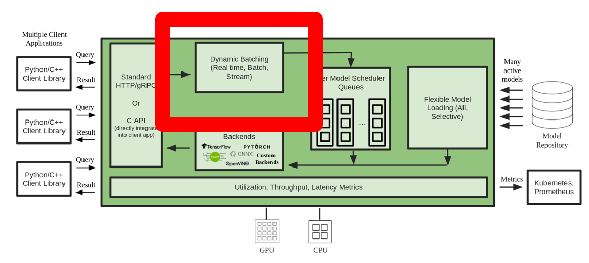
Many practitioners tend to run inference sequentially when the server is invoked with multiple independent requests. Although easier to set up, it’s usually not the best practice to utilize GPU’s compute power. To address this, Triton offers the built-in optimizations of dynamic batching to combine these independent inference requests on the server side to form a larger batch dynamically to increase throughput. The following diagram illustrates the Triton runtime architecture.
In the preceding architecture, all the requests reach the dynamic batcher first before entering the actual model scheduler queues to wait for inference. You can set your preferred batch sizes for dynamic batching using the preferred_batch_size settings in the model configuration. (Note that the formed batch size needs to be less than the max_batch_size the model supports.) You can also configure max_queue_delay_microseconds to specify the maximum delay time in the batcher to wait for other requests to join the batch based on your latency requirements.
The following code snippet shows how you can add this feature with model configuration files to set dynamic batching with a preferred batch size of 16 for the actual inference. With the current settings, the model instance is invoked instantly when the preferred batch size of 16 is met or the delay time of 100 microseconds has elapsed since the first request reached the dynamic batcher.
Running models concurrently
Another essential optimization offered in Triton to maximize hardware utilization without additional latency overhead is concurrent model execution, which allows multiple models or multiple copies of the same model to run in parallel. This feature enables Triton to handle multiple inference requests simultaneously, which increases the inference throughput by utilizing otherwise idle compute power on the hardware.
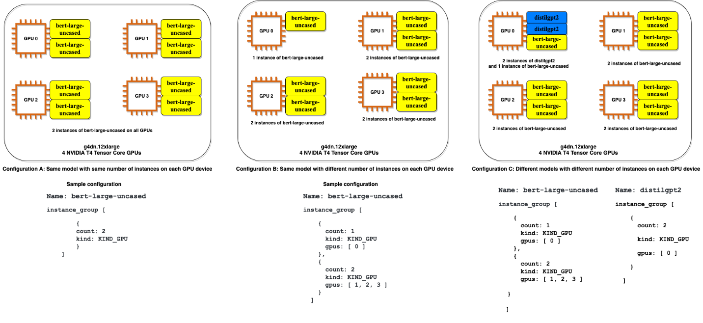
The following figure showcases how you can easily configure different model deployment policies with only a few lines of code changes. For example, configuration A (left) shows that you can broadcast the same configuration of two model instances of bert-large-uncased to all available GPUs. In contrast, configuration B (middle) shows a different configuration for GPU 0 only, without changing the policies on the other GPUs. You can also deploy instances of different models on a single GPU, as shown in configuration C (right).
In configuration C, the compute instance can handle two concurrent requests for the DistilGPT-2 model and seven concurrent requests for the bert-large-uncased model in parallel. With these optimizations, the hardware resources can be better utilized for the serving process, thereby improving the throughput and providing better cost-efficiency for your workload.
TensorRT
NVIDIA TensorRT is an SDK for high-performance deep learning inference that works seamlessly with Triton. TensorRT, which supports every major deep learning framework, includes an inference optimizer and runtime that delivers low latency and high throughput to run inferences with massive volumes of data via powerful optimizations.
TensorRT optimizes the graph to minimize memory footprint by freeing unnecessary memory and efficiently reusing it. Additionally, TensorRT compilation fuses the sparse operations inside the model graph to form a larger kernel to avoid the overhead of multiple small kernel launches. Kernel auto-tuning helps you fully utilize the hardware by selecting the best algorithm on your target GPU. CUDA streams enable models to run in parallel to maximize your GPU utilization for best performance. Last but not least, the quantization technique can fully use the mixed-precision acceleration of the Tensor cores to run the model in FP32, TF32, FP16, and INT8 to achieve the best inference performance.
Triton on SageMaker hosting
SageMaker hosting services are the set of SageMaker features aimed at making model deployment and serving easier. It provides a variety of options to easily deploy, auto scale, monitor, and optimize ML models tailored for different use cases. This means that you can optimize your deployments for all types of usage patterns, from persistent and always available with serverless options, to transient, long-running, or batch inference needs.
Under the SageMaker hosting umbrella is also the set of SageMaker inference Deep Learning Containers (DLCs), which come prepackaged with the appropriate model server software for their corresponding supported ML framework. This enables you to achieve high inference performance with no model server setup, which is often the most complex technical aspect of model deployment and in general, isn’t part of a data scientist’s skill set. Triton inference server is now available on SageMaker Deep Learning Containers (DLC).
This breadth of options, modularity, and ease of use of different serving frameworks makes SageMaker and Triton a powerful match.
SageMaker Inference Recommender for benchmarking test results
We use SageMaker Inference Recommender to run our experiments. SageMaker Inference Recommender offers two types of jobs: default and advanced, as illustrated in the following diagram.
The default job provides recommendations on instance types with just the model and a sample payload to benchmark. In addition to instance recommendations, the service also offers runtime parameters that improve performance. The default job’s recommendations are intended to narrow down the instance search. In some cases, it could be the instance family, and in others, it could be the specific instance types. The results of the default job are then fed into the advanced job.
The advanced job offers more controls to further fine-tune performance. These controls simulate the real environment and production requirements. Among these controls is the traffic pattern, which aims to stage the request pattern for the benchmarks. You can set ramps or steady traffic by using the traffic pattern’s multiple phases. For example, an InitialNumberOfUsers of 1, SpawnRate of 1, and DurationInSeconds of 600 may result in ramp traffic of 10 minutes with 1 concurrent user at the beginning and 10 at the end. Additionally, on the controls, MaxInvocations and ModelLatencyThresholds set the threshold of production, so when one of the thresholds is exceeded, the benchmarking stops.
Finally, recommendation metrics include throughput, latency at maximum throughput, and cost per inference, so it’s easy to compare them.
We use the advanced job type of SageMaker Inference Recommender to run our experiments to gain additional control over the traffic patterns, and fine-tune the configuration of the serving container.
Experiment setup
We use the custom load test feature of SageMaker Inference Recommender to benchmark the NLP profile outlined in our use case. We first define the following prerequisites related to the NLP model and ML task. SageMaker Inference Recommender uses this information to pull an inference Docker image from Amazon Elastic Container Registry (Amazon ECR) and register the model with the SageMaker model registry.
| Domain | NATURAL_LANGUAGE_PROCESSING |
| Task | FILL_MASK |
| Framework | PYTORCH: 1.6.0 |
| Model | bert-large-uncased |
The traffic pattern configurations in SageMaker Inference Recommender allow us to define different phases for the custom load test. The load test starts with two initial users and spawns two new users every minute, for a total duration of 25 minutes (1500 seconds), as shown in the following code:
We experiment with load testing the same model in two different states. The PyTorch-based experiments use the standard, unaltered PyTorch model. For the TensorRT-based experiments, we convert the PyTorch model into a TensorRT engine beforehand.
We apply different combinations of the performance optimization features on these two models, summarized in the following table.
| Configuration Name | Configuration Description | Model Configuration |
pt-base |
PyTorch baseline | Base PyTorch model, no changes |
pt-db |
PyTorch with dynamic batching | dynamic_batching
{} |
pt-ig |
PyTorch with multiple model instances | instance_group [
{
count: 2
kind: KIND_GPU
}
] |
pt-ig-db |
PyTorch with multiple model instances and dynamic batching | dynamic_batching
{},
instance_group [
{
count: 2
kind: KIND_GPU
}
] |
trt-base |
TensorRT baseline | PyTorch model compiled with TensoRT trtexec utility |
trt-db |
TensorRT with dynamic batching | dynamic_batching
{} |
trt-ig |
TensorRT with multiple model instances | instance_group [
{
count: 2
kind: KIND_GPU
}
] |
trt-ig-db |
TensorRT with multiple model instances and dynamic batching | dynamic_batching
{},
instance_group [
{
count: 2
kind: KIND_GPU
}
] |
Test results and observations
We conducted load tests for three instance types within the same g4dn family: ml.g4dn.xlarge, ml.g4dn.2xlarge and ml.g4dn.12xlarge. All g4dn instance types have access to NVIDIA T4 Tensor Core GPUs, and 2nd Generation Intel Cascade Lake processors. The logic behind the choice of instance types was to have both an instance with only one GPU available, as well as an instance with access to multiple GPUs—four in the case of ml.g4dn.12xlarge. Additionally, we wanted to test if increasing the vCPU capacity on the instance with only one available GPU would yield a cost-performance ratio improvement.
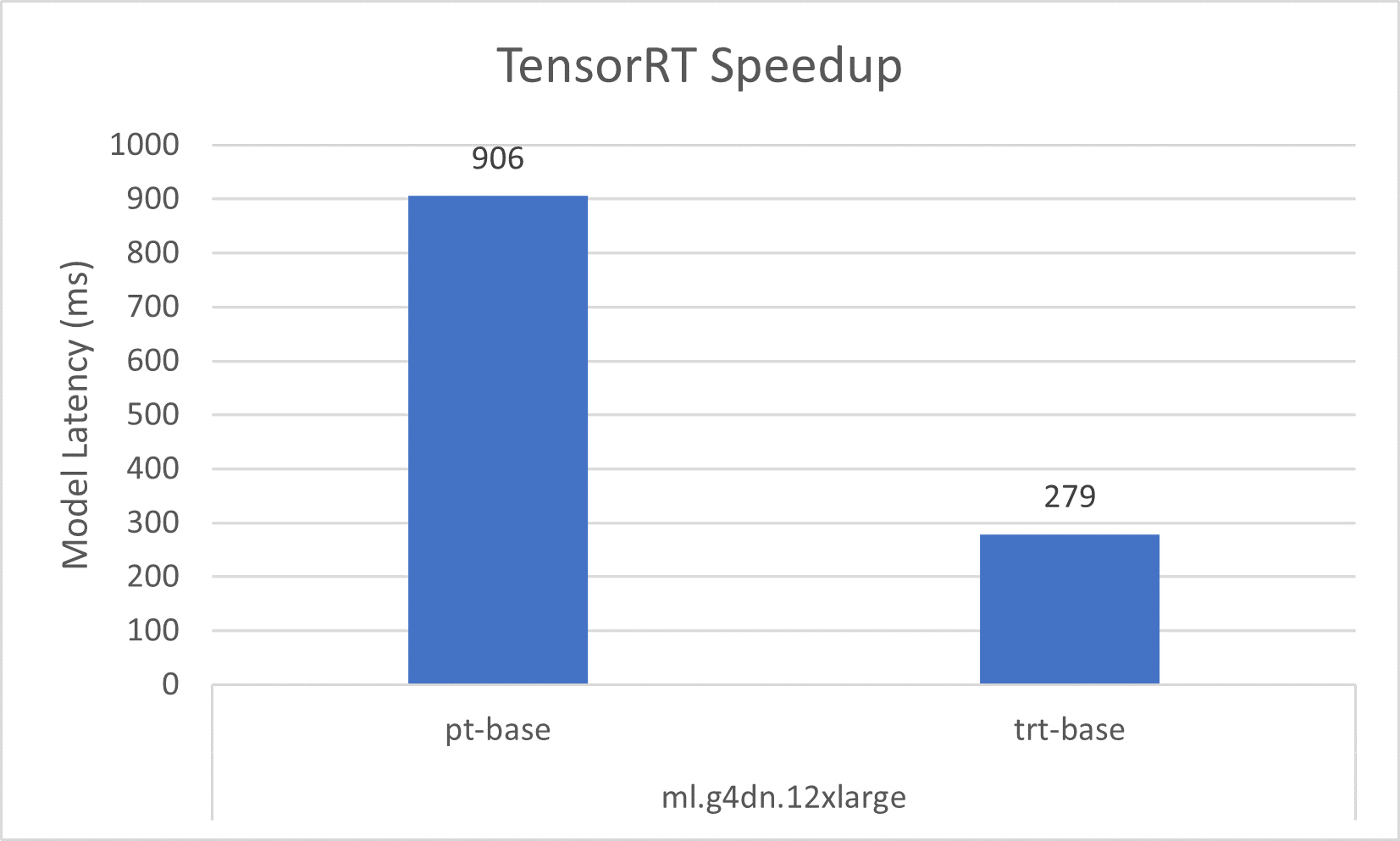
Let’s go over the speedup of the individual optimization first. The following graph shows that TensorRT optimization provides a 50% reduction in model latency compared to the native one in PyTorch on the ml.g4dn.xlarge instance. This latency reduction grows to over three times on the multi-GPU instances of ml.g4dn.12xlarge. Meanwhile, the 30% throughput improvement is consistent on both instances, resulting in better cost-effectiveness after applying TensorRT optimizations.
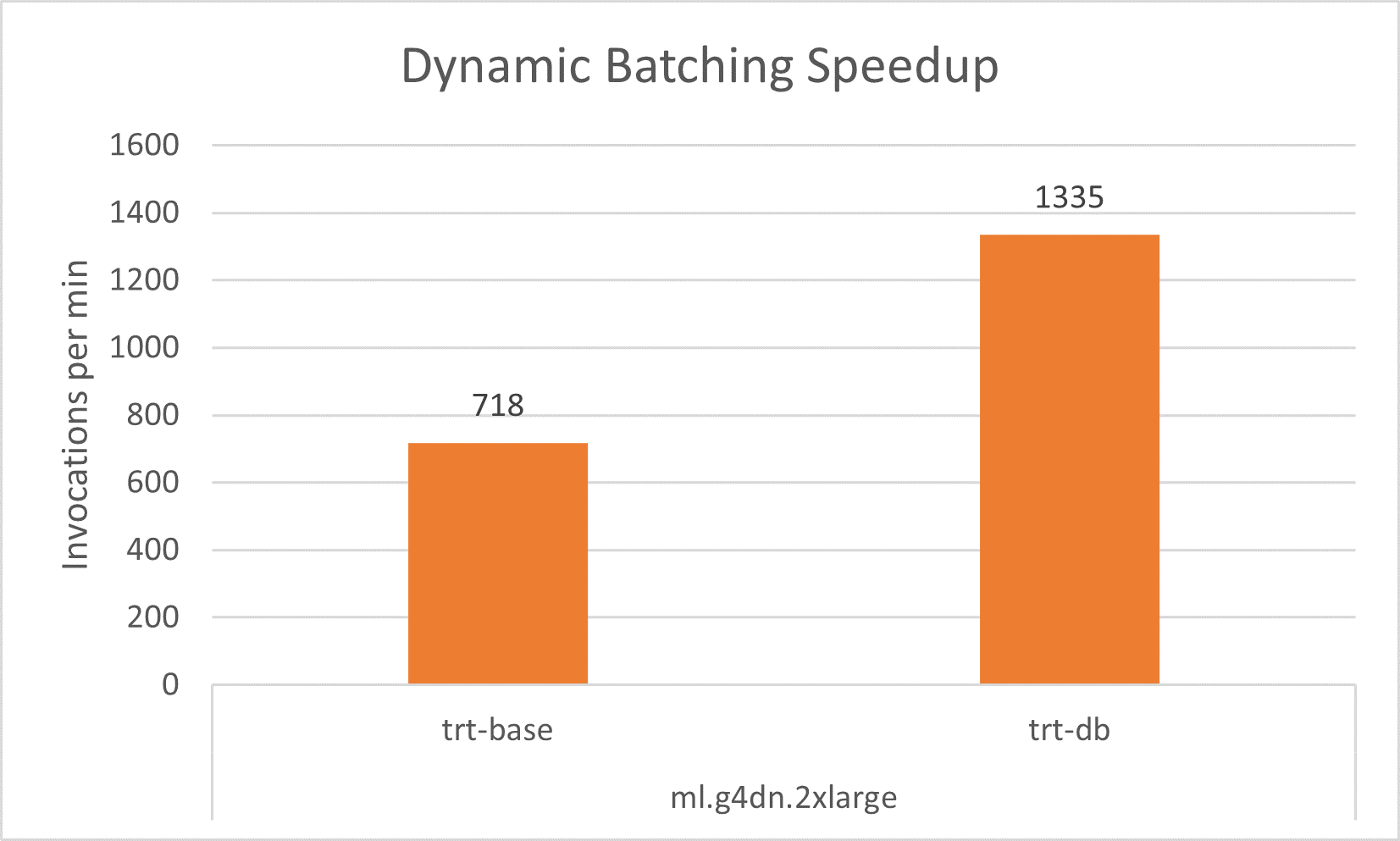
With dynamic batching, we can get close to 2x improvement in throughput using the same hardware architecture on all experiments instance of ml.g4dn.xlarge, ml.g4dn.2xlarge and ml.g4dn.12xlarge without noticeable latency increase.
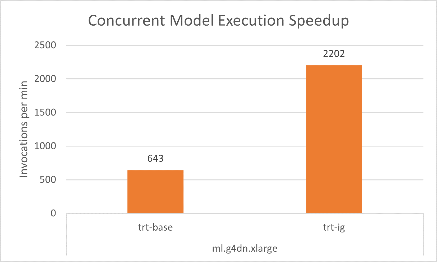
Similarly, concurrent model execution enable us to obtain about 3-4x improvement in throughput by maximizing the GPU utilization on ml.g4dn.xlarge instance and about 2x improvement on both the ml.g4dn.2xlarge instance and the multi-GPU instance of ml.g4dn.12xlarge.. This throughput increase comes without any overhead in the latency.
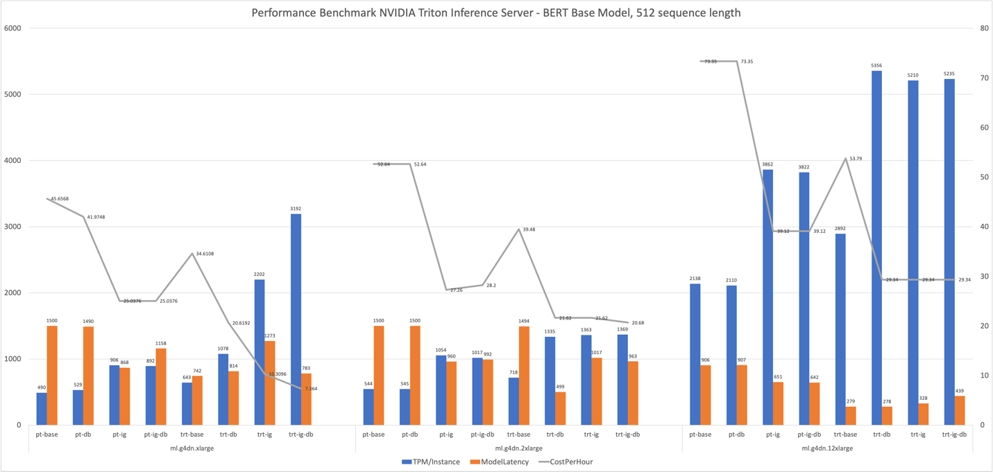
Better still, we can integrate all these optimizations to provide the best performance by utilizing the hardware resources to the fullest. The following table and graphs summarize the results we obtained in our experiments.
| Configuration Name | Model optimization |
Dynamic Batching |
Instance group config | Instance type | vCPUs | GPUs |
GPU Memory (GB) |
Initial Instance Count[1] | Invocations per min per Instance | Model Latency | Cost per Hour[2] |
| pt-base | NA | No | NA | ml.g4dn.xlarge | 4 | 1 | 16 | 62 | 490 | 1500 | 45.6568 |
| pt-db | NA | Yes | NA | ml.g4dn.xlarge | 4 | 1 | 16 | 57 | 529 | 1490 | 41.9748 |
| pt-ig | NA | No | 2 | ml.g4dn.xlarge | 4 | 1 | 16 | 34 | 906 | 868 | 25.0376 |
| pt-ig-db | NA | Yes | 2 | ml.g4dn.xlarge | 4 | 1 | 16 | 34 | 892 | 1158 | 25.0376 |
| trt-base | TensorRT | No | NA | ml.g4dn.xlarge | 4 | 1 | 16 | 47 | 643 | 742 | 34.6108 |
| trt-db | TensorRT | Yes | NA | ml.g4dn.xlarge | 4 | 1 | 16 | 28 | 1078 | 814 | 20.6192 |
| trt-ig | TensorRT | No | 2 | ml.g4dn.xlarge | 4 | 1 | 16 | 14 | 2202 | 1273 | 10.3096 |
| trt-db-ig | TensorRT | Yes | 2 | ml.g4dn.xlarge | 4 | 1 | 16 | 10 | 3192 | 783 | 7.364 |
| pt-base | NA | No | NA | ml.g4dn.2xlarge | 8 | 1 | 32 | 56 | 544 | 1500 | 52.64 |
| pt-db | NA | Yes | NA | ml.g4dn.2xlarge | 8 | 1 | 32 | 59 | 517 | 1500 | 55.46 |
| pt-ig | NA | No | 2 | ml.g4dn.2xlarge | 8 | 1 | 32 | 29 | 1054 | 960 | 27.26 |
| pt-ig-db | NA | Yes | 2 | ml.g4dn.2xlarge | 8 | 1 | 32 | 30 | 1017 | 992 | 28.2 |
| trt-base | TensorRT | No | NA | ml.g4dn.2xlarge | 8 | 1 | 32 | 42 | 718 | 1494 | 39.48 |
| trt-db | TensorRT | Yes | NA | ml.g4dn.2xlarge | 8 | 1 | 32 | 23 | 1335 | 499 | 21.62 |
| trt-ig | TensorRT | No | 2 | ml.g4dn.2xlarge | 8 | 1 | 32 | 23 | 1363 | 1017 | 21.62 |
| trt-db-ig | TensorRT | Yes | 2 | ml.g4dn.2xlarge | 8 | 1 | 32 | 22 | 1369 | 963 | 20.68 |
| pt-base | NA | No | NA | ml.g4dn.12xlarge | 48 | 4 | 192 | 15 | 2138 | 906 | 73.35 |
| pt-db | NA | Yes | NA | ml.g4dn.12xlarge | 48 | 4 | 192 | 15 | 2110 | 907 | 73.35 |
| pt-ig | NA | No | 2 | ml.g4dn.12xlarge | 48 | 4 | 192 | 8 | 3862 | 651 | 39.12 |
| pt-ig-db | NA | Yes | 2 | ml.g4dn.12xlarge | 48 | 4 | 192 | 8 | 3822 | 642 | 39.12 |
| trt-base | TensorRT | No | NA | ml.g4dn.12xlarge | 48 | 4 | 192 | 11 | 2892 | 279 | 53.79 |
| trt-db | TensorRT | Yes | NA | ml.g4dn.12xlarge | 48 | 4 | 192 | 6 | 5356 | 278 | 29.34 |
| trt-ig | TensorRT | No | 2 | ml.g4dn.12xlarge | 48 | 4 | 192 | 6 | 5210 | 328 | 29.34 |
| trt-db-ig | TensorRT | Yes | 2 | ml.g4dn.12xlarge | 48 | 4 | 192 | 6 | 5235 | 439 | 29.34 |
[1] Initial instance count in the above table is the recommended number of instances to use with an autoscaling policy to maintain the throughput and latency requirements for your workload.
[2] Cost per hour in the above table is calculated based on the Initial instance count and price for the instance type.
Results mostly validate the impact that was expected of different performance optimization features:
- TensorRT compilation has the most reliable impact across all instance types. Transactions per minute per instance increased by 30–35%, with a consistent cost reduction of approximately 25% when compared to the TensorRT engine’s performance to the default PyTorch BERT (
pt-base). The increased performance of the TensorRT engine is compounded upon and exploited by the other tested performance tuning features. - Loading two models on each GPU (instance group) almost strictly doubled all measured metrics. Invocations per minute per instance increased approximately 80–90%, yielding a cost reduction in the 50% range, almost as if we were using two GPUs. In fact, Amazon CloudWatch metrics for our experiments on g4dn.2xlarge (as an example) confirms that both CPU and GPU utilization double when we configure an instance group of two models.
Further performance and cost-optimization tips
The benchmark presented in this post just scratched the surface of the possible features and techniques that you can use with Triton to improve inference performance. These range from data preprocessing techniques, such as sending binary payloads to the model server or payloads with bigger batches, to native Triton features, such as the following:
- Model warmup, which prevents initial, slow inference requests by completely initializing the model before the first inference request is received.
- Response cache, which caches repeated requests.
- Model ensembling, which enables you to create a pipeline of one or more models and the connection of input and output tensors between those models. This opens the possibility of adding preprocessing and postprocessing steps, or even inference with other models, to the processing flow for each request.
We expect to test and benchmark these techniques and features in a future post, so stay tuned!
Conclusion
In this post, we explored a few parameters that you can use to maximize the performance of your SageMaker real-time endpoint for serving PyTorch BERT models with Triton Inference Server. We used SageMaker Inference Recommender to perform the benchmarking tests to fine-tune these parameters. These parameters are in essence related to TensorRT-based model optimization, leading to almost 50% improvement in response times compared to the non-optimized version. Additionally, running models concurrently and using dynamic batching of Triton led to almost a 70% increase in throughput. Fine-tuning these parameters led to an overall reduction of inference cost as well.
The best way to derive the correct values is through experimentation. However, to start building empirical knowledge on performance tuning and optimization, you can observe the combinations of different Triton-related parameters and their effect on performance across ML models and SageMaker ML instances.
SageMaker provides the tools to remove the undifferentiated heavy lifting from each stage of the ML lifecycle, thereby facilitating the rapid experimentation and exploration needed to fully optimize your model deployments.
You can find the notebook used for load testing and deployment on GitHub. You can update Triton configurations and SageMaker Inference Recommender settings to best fit your use case to achieve cost-effective and best-performing inference workloads.
About the Authors
 Vikram Elango is an AI/ML Specialist Solutions Architect at Amazon Web Services, based in Virginia USA. Vikram helps financial and insurance industry customers with design, thought leadership to build and deploy machine learning applications at scale. He is currently focused on natural language processing, responsible AI, inference optimization and scaling ML across the enterprise. In his spare time, he enjoys traveling, hiking, cooking and camping with his family.
 João Moura is an AI/ML Specialist Solutions Architect at Amazon Web Services. He mostly focuses on NLP use-cases and helping customers optimize Deep Learning model training and deployment. He is also an active proponent of low-code ML solutions and ML-specialized hardware.
 Mohan Gandhi is a Senior Software Engineer at AWS. He has been with AWS for the last 9 years and has worked on various AWS services like EMR, EFA and RDS on Outposts. Currently, he is focused on improving the SageMaker Inference Experience. In his spare time, he enjoys hiking and running marathons.
 Dhawal Patel is a Principal Machine Learning Architect at AWS. He has worked with organizations ranging from large enterprises to mid-sized startups on problems related to distributed computing, and Artificial Intelligence. He focuses on Deep learning including NLP and Computer Vision domains. He helps customers achieve high performance model inference on SageMaker.
 Santosh Bhavani is a Senior Technical Product Manager with the Amazon SageMaker Elastic Inference team. He focuses on helping SageMaker customers accelerate model inference and deployment. In his spare time, he enjoys traveling, playing tennis, and drinking lots of Pu’er tea.
 Jiahong Liu is a Solution Architect on the Cloud Service Provider team at NVIDIA. He assists clients in adopting machine learning and AI solutions that leverage NVIDIA accelerated computing to address their training and inference challenges. In his leisure time, he enjoys origami, DIY projects, and playing basketball.

