AWS Machine Learning Blog
Unified data preparation and model training with Amazon SageMaker Data Wrangler and Amazon SageMaker Autopilot – Part 1
September 2023: This post was reviewed and updated for accuracy.
Data fuels machine learning (ML); the quality of data has a direct impact on the quality of ML models. Therefore, improving data quality and employing the right feature engineering techniques are critical to creating accurate ML models. ML practitioners often tediously iterate on feature engineering, choice of algorithms, and other aspects of ML in search of optimal models that generalize well on real-world data and deliver the desired results. Because speed in doing business disproportionately matters, this extremely tedious and iterative process may lead to project delays and lost business opportunities.
Amazon SageMaker Data Wrangler reduces the time to aggregate and prepare data for ML from weeks to minutes, and Amazon SageMaker Autopilot automatically builds, trains, and tunes the best ML models based on your data. With Autopilot, you still maintain full control and visibility of your data and model. Both services are purpose-built to make ML practitioners more productive and accelerate time to value.
Data Wrangler now provides a unified experience enabling you to prepare data and seamlessly train a ML model in Autopilot. With this newly launched feature, you can now prepare your data in Data Wrangler and easily launch Autopilot experiments directly from the Data Wrangler user interface (UI). With just a few clicks, you can automatically build, train, and tune ML models, making it easier to employ state-of-the-art feature engineering techniques, train high-quality ML models, and gain insights from your data faster.
In this post, we discuss how you can use this new integrated experience in Data Wrangler to analyze datasets and easily build high-quality ML models in Autopilot.
Dataset overview
Pima Indians are an Indigenous group that live in Mexico and Arizona, US. Studies show Pima Indians as a high-risk population group for diabetes mellitus. Predicting the probability of an individual’s risk and susceptibility to a chronic illness like diabetes is an important task in improving the health and well-being of this often underrepresented minority group.
We use the Pima Indian Diabetes public dataset to predict the susceptibility of an individual to diabetes. We focus on the new integration between Data Wrangler and Autopilot to prepare data and automatically create an ML model without writing a single line of code.
The dataset contains information about Pima Indian females 21 years or older and includes several medical predictor (independent) variables and one target (dependent) variable, Outcome. The following chart describes the columns in our dataset.
| Column Name | Description |
| Pregnancies | The number of times pregnant |
| Glucose | Plasma glucose concentration in an oral glucose tolerance test within 2 hours |
| BloodPressure | Diastolic blood pressure (mm Hg) |
| SkinThickness | Triceps skin fold thickness (mm) |
| Insulin | 2-hour serum insulin (mu U/ml) |
| BMI | Body mass index (weight in kg/(height in m)^2) |
| DiabetesPedigree | Diabetes pedigree function |
| Age | Age in years |
| Outcome | The target variable |
The dataset contains 768 records, with 9 total features. We store this dataset in Amazon Simple Storage Bucket (Amazon S3) as a CSV file and then import the CSV directly into a Data Wrangler flow from Amazon S3.
Solution overview
The following diagram summarizes what we accomplish in this post.
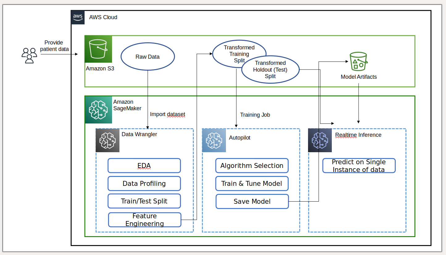
Data scientists, doctors, and other medical domain experts provide patient data with information on glucose levels, blood pressure, body mass index, and other features used to predict the likelihood of having diabetes. With the dataset in Amazon S3, we import the dataset into Data Wrangler to perform exploratory data analysis (EDA), data profiling. After splitting the dataset into train and test portions for model building and model evaluation, we then perform feature engineering on the training split.
We then use Autopilot’s new feature integration to quickly build a model directly from the Data Wrangler interface. We choose Autopilot’s best model based on the model with the highest F-beta score. After Autopilot finds the best model, we run a SageMaker Batch Transform job on the test (holdout) set with the model artifacts of the best model for evaluation.
Medical experts can provide new data to the validated model to obtain a prediction to see if a patient will likely have diabetes. With these insights, medical experts can start treatment early to improve the health and well-being of vulnerable populations. Medical experts can also explain a model’s prediction by referencing the model’s detail in Autopilot because they have full visibility into the model’s explainability, performance, and artifacts. This visibility in addition to validation of the model from the test set gives medical experts greater confidence in the model’s predictive ability.
We walk you through the following high-level steps.
- Import the dataset from Amazon S3.
- Perform EDA and data profiling with Data Wrangler.
- Split data into train and test sets.
- Perform feature engineering to handle outliers and missing values.
- Train and build a model with Autopilot.
- Test the model on a holdout sample with a SageMaker notebook.
- Analyze validation and test set performance.
Prerequisites
Complete the following prerequisite steps:
- Upload the dataset to an S3 bucket of your choice.
- Make sure you have the necessary permissions. For more information, refer to Get Started with Data Wrangler.
- Set up a SageMaker domain configured to use Data Wrangler. For instructions, refer to Onboard to Amazon SageMaker Domain.
Import your dataset with Data Wrangler
You can integrate a Data Wrangler data flow into your ML workflows to simplify and streamline data preprocessing and feature engineering using little to no coding. Complete the following steps:
- Create a new Data Wrangler flow.
If this is your first time opening Data Wrangler, you may have to wait a few minutes for it to be ready. - Choose the dataset stored in Amazon S3 and import it into Data Wrangler.
 After you import the dataset, you should see the beginnings of a data flow within the Data Wrangler UI. You now have a flow diagram.
 - Choose the plus sign next to Data types and choose Edit to confirm that Data Wrangler automatically inferred the correct data types for your data columns.

If the data types aren’t correct, you can easily modify them through the UI. If multiple data sources are present, you can join or concatenate them.
We can now create an analysis and add transformations.
Perform exploratory data analysis with the data insights report
Exploratory data analysis is a critical part of the ML workflow. We can use the new data insights report from Data Wrangler to gain a better understanding of the profile and distribution of our data. The report includes summary statistics, data quality warnings, target column insights, a quick model, and information about anomalous and duplicate rows.
- Choose the plus sign next to Data types and choose Get data insights.

- For Analysis Name (Optional) type EDA.
- For Target column, choose Outcome.
- For Problem type, and (optionally) select Classification.
- Choose Create.

The results show a summary data with the dataset statistics.

We can also view the distribution of the labeled rows with a histogram, an estimate of the expected predicted quality of the model with the quick model feature, and a feature summary table.


We don’t go into the details of analyzing the data insights report; refer to Accelerate data preparation with data quality and insights in Amazon SageMaker Data Wrangler for additional details about how you can use the data insights report to accelerate your data preparation steps.
Now that we’ve performed some data analysis, we’re ready to split our dataset into training and testing before we build a model.
Split data into training and testing
In the model building phase of your ML workflow, you test the efficacy of your model by running batch predictions. You can set aside a testing (or holdout) dataset for evaluation to see how your model performs by comparing the predictions to the ground truth. Generally, if more of the model’s predictions match the true labels, we can determine the model is performing well.
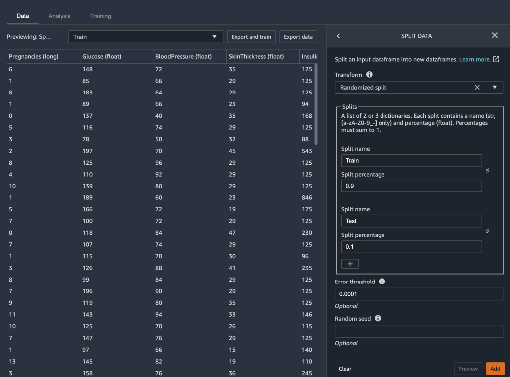
We use Data Wrangler to split our dataset for testing. We retain 90% of our dataset for training because we have a relatively small dataset. The remaining 10% of our dataset serves as the test dataset. We use this dataset to validate the Autopilot model later in this post.
We split our data by:
- Choose Add Transform from the Data types node
- Add Step. Choose Split Data.
- Choose Randomized split as the transform. We designate 9 as the split percentage for training and 0.1 for testing.
Perform feature engineering
Now that we’ve profiled and analyzed the distribution of our input columns at a high level, the first consideration for improving the quality of our data could be to handle missing values.
For example, we know that zeros (0) for the Insulin column represent missing values. We could follow the recommendation to replace the zeros with NaN. But on closer examination, we find that the minimum value is 0 for others columns such as Glucose, BloodPressure, SkinThickness, and BMI. We need a way to handle missing values, but need to be sensitive to columns with zeros as valid data. Let’s see how we can fix this.
In the Feature Details section, the report raises a Disguised missing value warning for the feature Insulin.

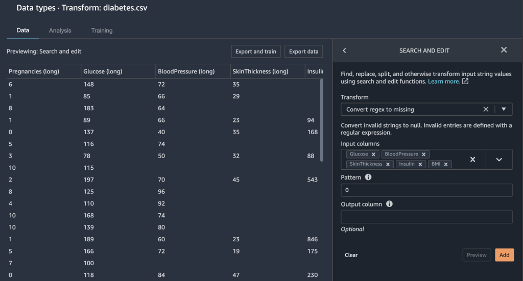
Because zeros in the Insulin column are in fact missing data, we use the Convert regex to missing transform to transform zero values to empty (missing values).
- Choose the plus sign next to the Train Dataset and choose Add transform. (NOTE: You can double-click on either Dataset in the split to verify which is train and which is test if you aren’t sure.)
- Choose Search and edit.
- For Transform, choose Convert regex to missing.
- For Input columns, choose the columns
Insulin,Glucose,BloodPressure,SkinThickness, andBMI. - For Pattern, enter
0. - Click Preview and Add to save this step.
The 0 entries underInsulin,Glucose,BloodPressure,SkinThickness, andBMIare now missing values.Data Wrangler gives you a few other options to fix missing values.
- We handle missing values by imputing the approximate median for the
Insulin,Glucose,BloodPressure,SkinThickness, andBMIcolumns. We also want to ensure that our features are on the same scale. We don’t want to accidentally give more weight to a certain feature just because they contain a larger numeric range. We normalize our features to do this.
 - Add a new Process numeric transform and choose Scale values.
- For Scaler, choose Min-max scaler.
- For Input columns, choose the columns
Pregnancies,BloodPressure,Glucose,SkinThickness,Insulin,BMI, andAge. - Set Min to
0and Max to1.
This makes sure that our features are between the values 0 and 1.

After performing these transformation steps, your flow should look similar to below (where the Test dataset is on the upper row, and the Train dataset is on the bottom row leading to the transform steps):
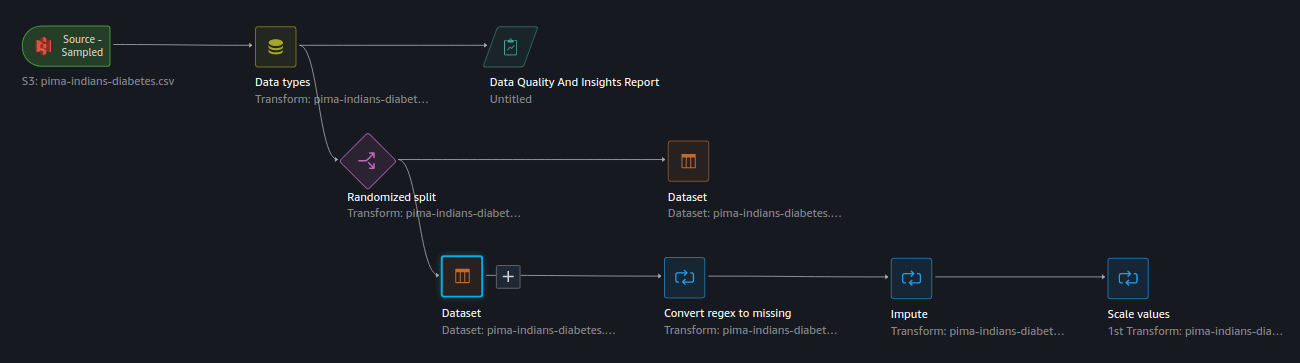
With the data transformation and featuring engineering steps complete, we’re now ready to train a model.
Export and Train the model
We can use the new Data Wrangler integration with Autopilot to directly train a model from the Data Wrangler data flow UI.
- Choose the plus sign next to the Scale values node, and choose Train model.
- For Amazon S3 location, specify the Amazon S3 location where SageMaker exports your data.
If presented with a root bucket path by default, Data Wrangler will create a unique export sub-directory under it — you don’t need to modify this default root path unless you’d like to.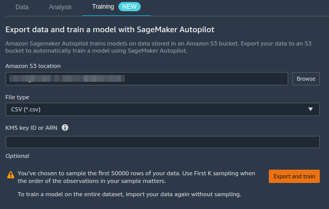 Autopilot uses this location to automatically train a model, saving you time from having to define the output location of the Data Wrangler flow, then having to define the input location of the Autopilot training data. This makes for a more seamless experience.
 - Click the Export and train button to export the transformed data to S3.
Once export is successful, you are taken to the Create an Autopilot experiment page, with the Input data S3 location already filled in for you (as it was populated from the results of the previous screen.)On this page, fill in: - An Experiment name (optionally, if you don’t want the default name.)
- Click Next: Target and features.

- Target (in our case, Outcome, as its the column we wish to predict).
- Then click Next: Training method.

- Leave the default selection of Auto, and click Next: Deployment and advanced settings to continue.
Lastly, we’re brought to the Deployment and advanced settings screen. - For Deployment option, choose Do not auto deploy best model (since in this blog post, we’ll be doing inference locally, not against an endpoint.)
- Click Next: Review and create to continue.

On the Review and create screen we see a summary of the settings chosen for our Autopilot experiment.

Click Create experiment to begin the model creation process.
At this point, we’re brought to the AutoPilot job description page. The models will display on the Models tab as they are generated. You’ll know the process has completed by inspecting the Job Profile tab, and looking for a Completed value for the Status field.
NOTE: To get back to this AutoPilot job description page at any time, from SageMaker Studio:
- Select AutoML from the Home.
- Select the name of the AutoPilot job you created in the experiments pane.
- Click on the experiment.
Test the model on a holdout sample
When AutoPilot completes the experiment, we can view the training results and explore the best model from the AutoPilot job description page.

Click on the Best model labeled model. Or select the Best model labeled model and click on Open in model details.
The Performance tab displays several model measurement tests, including a confusion matrix, the area under the precision/recall curve (AUCPR), and the area under the receiver operating characteristic curve (ROC). These illustrate the overall validation performance of the model, but they don’t tell us if the model will generalize well. We still need to run evaluations on unseen test data to see how accurately the model predicts if an individual will have diabetes.
Remember earlier on when we created the Train / Test split? We’ll use it now to verify the model can generalize well against against data it has never seen. To export the test data:
- Select the + next to the data flow’s Test dataset node.
- Select Add Destination → Amazon S3.
- Specify an Amazon S3 path you will export the data to. (Remember the path you exported to… we’ll refer to this path next when we perform inference.)
- Leave the other defaults as-is.
- Click Add Destination to export the data to S3.
Perform batch inferencing
Create a new SageMaker notebook to perform batch inferencing on the holdout sample and assess the test performance. Refer to the following GitHub repo for a sample notebook to run batch inference for validation.
NOTE: If you’re interested in performing realtime inference against an endpoint, we go over that as well in Part 2 of the series. Keep in mind however that in order to complete Part 2 of the series, this first part is a prerequisite.
Analyze validation and test set performance
When the batch transform is complete, we create a confusion matrix to compare the actual and predicted outcomes of the holdout dataset.
We see 23 true positives and 33 true negatives from our results. In our case, true positives refer to the model correctly predicting an individual as having diabetes. In contrast, true negatives refer to the model correctly predicting an individual as not having diabetes.
In our case, precision and recall are important metrics. Precision essentially measures all individuals predicted to have diabetes, how many really have diabetes? In contrast, recall helps measure all individual who indeed have diabetes, how many were predicted to have diabetes? For example, you may want to use a model with high precision because you want to treat as many individuals as you can, especially if the first stage of treatment has no effect on individuals without diabetes (these are false positives—those labeled as having it when in fact they do not).
We also plot the area under the ROC curve (AUC) graph to evaluate the results. The higher the AUC, the better the model is at distinguishing between classes, which in our case is how well the model performs at distinguishing patients with and without diabetes.
Conclusion
In this post, we demonstrated how to integrate your data processing, featuring engineering, and model building using Data Wrangler and Autopilot. We highlighted how you can easily train and tune a model with Autopilot directly from the Data Wrangler user interface. With this integration feature, we can quickly build a model after completing feature engineering, without writing any code. Then we referenced Autopilot’s best model to run batch predictions using the AutoML class with the SageMaker Python SDK.
Please join us in Part 2 as we use the Autopilot integration once again to train a model against the same training dataset, but instead of performing bulk inference, we perform real-time inference against an Amazon SageMaker inference endpoint that is created automatically for us.
Get started using Data Wrangler today to experience how easy it is to build ML models using SageMaker Autopilot.
About the Authors
 Peter Chung is a Solutions Architect for AWS, and is passionate about helping customers uncover insights from their data. He has been building solutions to help organizations make data-driven decisions in both the public and private sectors. He holds all AWS certifications as well as two GCP certifications. He enjoys coffee, cooking, staying active, and spending time with his family.
 Pradeep Reddy is a Senior Product Manager in the SageMaker Low/No Code ML team, which includes SageMaker Autopilot, SageMaker Automatic Model Tuner. Outside of work, Pradeep enjoys reading, running and geeking out with palm sized computers like raspberry pi, and other home automation tech.
 Arunprasath Shankar is an Artificial Intelligence and Machine Learning (AI/ML) Specialist Solutions Architect with AWS, helping global customers scale their AI solutions effectively and efficiently in the cloud. In his spare time, Arun enjoys watching sci-fi movies and listening to classical music.
 Srujan Gopu is a Senior Frontend Engineer in SageMaker Low Code/No Code ML helping customers of SageMaker Autopilot and SageMaker Canvas products. When not coding, Srujan enjoys going for a run with his dog Max, listening to audio books and VR game development.
 Geremy Cohen is a Solutions Architect with AWS where he helps customers build cutting-edge, cloud-based solutions. In his spare time, he enjoys short walks on the beach, exploring the bay area with his family, fixing things around the house, breaking things around the house, and BBQing.
 Shweta Thapa is a Solutions Architect in Enterprise Engaged at AWS and a member of Comprehend Champions. She enjoys helping her customers with their journey and growth in the cloud, listening to their business needs, and offering them the best solutions. In her free time, Shweta enjoys going out for a run, traveling, and most of all spending time with her baby daughter.