Best Practices from Onica for Optimizing Query Performance on Amazon Redshift

By Scott Peters, Lead Data Science Architect at Onica
By Sudhir Gupta, Sr. Partner Solutions Architect at AWS

Effective and economical use of data is critical to the success of companies across a broad array of industries. As data volumes increase exponentially, effectively managing and extracting value from data becomes increasingly difficult.

Getting the best performance out of your data platform also becomes more difficult as more and more business units with competing priorities are added to it.

Onica is an AWS Partner Network (APN) Premier Consulting Partner with AWS Competencies in Data & Analytics, Machine Learning, and Migration, among others. Onica is also a member of the AWS Managed Service Provider (MSP) Partner Program.

In this post, we discuss the best practices Onica has developed for using Amazon Redshift, the data warehouse of Amazon Web Services (AWS). No other data warehouse makes it as easy to gain new insights from all your data.

Data Lakes vs. Data Warehouses

There is often confusion about the difference between a data lake and data warehouse.

Data Lake

A data lake is a centralized repository that stores your structured and unstructured data at any scale. It is a complete archive of data collected over time.

A data lake accepts data from many sources, and stores it in a way that makes later processing and analysis easier. Incoming data is typically stored in as-close-to-raw form as possible, and then transformed and compressed.

Amazon Simple Storage Service (Amazon S3) is a typical data lake service. It provides secure and reliable low-cost storage at exabyte scale.

Data Warehouse

Whereas a data lake archives all data regardless of form or state, a data warehouse stores data in a reconciled state optimized for ongoing analytics and business intelligence operations.

Only the portion of data required for analytics is loaded from the data lake into the data warehouse, where complex joins and queries can be performed.

Amazon Redshift is a fast, petabyte-scale cloud data warehouse service used by tens of thousands of customers. Amazon Redshift is also integrated with Amazon S3, AWS Glue, AWS Identity and Access Management (IAM), Amazon EMR, Amazon QuickSight, AWS Lake Formation, and other AWS services.

Amazon Redshift Spectrum, a feature of Amazon Redshift, queries exabytes of data directly in an Amazon S3 data lake, with no data loading. The data can be stored in open file formats such as Parquet, JSON, and CSV.

 The Lake House Approach

Amazon Redshift enables customers to directly query and join data across both their data warehouse and S3 data lake. The lake house approach provides multiple benefits.

It enables querying of exabyte-scale data lakes in a high-performance, cost-effective way. It reduces data redundancy, as there is reduced need to copy data from the lake into the warehouse. It eliminates simple extract, transform, load (ETL) jobs, and related monitoring and maintenance overhead.

Data governance is also streamlined in a lake house approach because fewer data locations and tools reduce the number of permissions to manage. All of this reduces operational resources and maintenance effort, lowering overall operational cost.

Amazon Redshift Architecture in a Nutshell

Amazon Redshift architecture supports massively parallel processing (MPP). In essence, MPP distributes a job across multiple compute nodes that can process their portion simultaneously. MPP makes it possible to process complex queries on big data sets fast.

Amazon Redshift nodes are grouped into clusters. Each cluster has three types of nodes:

• Leader Node
  • Manages connections
  • SQL endpoint
  • Coordinates parallel SQL processing
• Compute Nodes
  • Comprised of “slices”
  • Columnar storage
  • Execute queries in parallel
• Amazon Redshift Spectrum Nodes
  • Execute queries against Amazon S3 data lake

Figure 1 – Nodes and clusters in Amazon Redshift architecture.

An Amazon Redshift cluster may have between 1-128 compute nodes. Each is partitioned into slices, which contain the table data and form a local processing zone.

Data on Amazon Redshift is stored in a columnar format, in 1MB immutable blocks. Each slice stores blocks in a range of values for each column.

Figure 2 – Column vs. row storage in Amazon Redshift.

How to Optimize Query Performance

Getting the best performance from Amazon Redshift typically comes down to optimizing the physical layout of data in the cluster to harmonize with your query patterns. When you don’t get the performance you expect from Amazon Redshift, try these changes:

• Reconfigure workload management
• Refine data distribution
• Refine data sorting

Reconfiguring Workload Management (WLM)

Customers often leave workload management (WLM) in its default configuration. In other words, Amazon Redshift assigns all queries against a cluster to the default queues, one for super user and one for user.

You may be able to improve performance by tuning WLM. You can do this in an automated or manual fashion.

With automatic WLM, Amazon Redshift manages concurrency and memory usage for you. You can create up to eight queues, each with its own priority. Amazon Redshift manages query concurrency based on resource usage within the cluster.

Manual WLM gives you additional control over the number of queues and their configuration. To modify a WLM queue, you can adjust the number of concurrent queries, memory allocation, and targets.

You can also optimize query throughout by enabling these WLM configuration parameters:

• Query monitoring rules
• Short query acceleration
• Concurrency scaling

Here’s how you can modify each parameter.

Query Monitoring Rules (QMR)

You can use query monitoring rules (QMR) to manage expensive or runaway queries. They are metrics-based boundaries for queries that run in any WLM queue. You can define a maximum of 25 QMR rules across all queues, and specify one of four actions to take if the rule triggers:

• LOG — Log query info in the STL_WLM_RULE_ACTION table.
• ABORT — Log the action and terminate the query.
• HOP — Log the action and move the query to a different queue if one exists, or terminate.
• PRIORITY — Change query priority (automated WLM only).

Short Query Acceleration (SQA)

Short query acceleration (SQA) prioritizes selected short-running queries ahead of longer-running queries. It uses machine learning algorithms to predict the execution time of a query, and runs short-running queries into a dedicated space for immediate processing.

Concurrency Scaling

When concurrency scaling is enabled, Amazon Redshift automatically adds multiple transient clusters to enable an increase in concurrent read queries. This happens in seconds, and provides consistently fast performance.

WLM Best Practices

For best results with WLM tuning, follow these best practices:

• Create separate WLM queues for different workload types.
• To avoid unused resources, keep the number of queues to a minimum (typically three or less).
• To maximize throughput, limit maximum total concurrency for the main cluster to 15 or less.
• Enable concurrency scaling to handle spiky concurrent read queries.
• Configure QMR rules and enable SQA.
• Leave a buffer of 5 percent of memory un-allocated for manual WLM configuration.
• Use different WLM setups for periodic workload pattern changes, such as increasing memory for the load/ETL queue during overnight load periods.

Refine Data Distribution

Amazon Redshift automatically distributes the rows of a table across the node slices according to the distribution style, which can be:

• AUTO — Default option. Starts the table with ALL, but switches to EVEN as the table grows.
• ALL — Full table is placed on the first slice of each compute node.
• EVEN — Round-robin distribution across slices.
• KEY — A column value is hashed, and the same hash value is placed on the same slice.

Use the appropriate distribution style to maximize the performance of JOIN, GROUP BY, and INSERT INTO SELECT operations. Also consider query patterns and table type to determine the best distribution style for your usage.

Take the following considerations into account when choosing the distribution style for a particular table:

• ALL
  • Small tables that are frequently joined and infrequently modified
  • Reference data or dimension tables
• EVEN
  • Tables not frequently joined or aggregated
  • Standalone fact tables
  • Large tables with obvious distribution key candidates
• KEY
  • Tables that are frequently joined
  • Fact tables or large dimension tables
• AUTO
  • When there is no clear choice between KEY and ALL distribution

Refine Data Sorting

Sort keys define the physical order of data on disk. Columns used in WHERE clause predicates are typically good choices for sort keys. Date- or time-related columns are common choices. Compound keys should not comprise more than four columns; more columns in a sort key increase overhead and result in marginal gains.

If your table is frequently joined, include the DISTKEY in the sort key and the first column.

Zone maps are minimum and maximum values for each block of data. They allow you to block-prune data not needed for a query. Zone maps are stored in memory and automatically generated.

In combination with zone maps, sort keys restrict scans to the minimally required number of blocks. The diagram below illustrates the effects of table sorting resulting in co-located data for time-based queries.

Figure 3 – Effect of table sorting resulting in co-located data for time-based queries.

Best Practices for Optimal Query Performance

To improve the performance of your queries, follow these best practices:

• Use SORT keys on columns often used in WHERE clause filters.
• Use DISTKEY on a column often used in JOIN predicates.
• Compress all columns except the first sort key column.
• Partition your data based upon the query filters, such as access pattern, in the data lake.
• Compress and use columnar file format, such as Parquet, as much as possible.
• Choose optimal file sizes to reduce Amazon S3 roundtrips (we recommend 100MB – 1GB).
• Ensure your use of standard date element ordering conforms to ISO standard (do not use dd-mm-yyyy format in an ORDER BY clause).
• Follow Amazon Redshift Advisor output to optimize the cluster performance by adopting recommended changes, such as changing distribution style, sort keys, WLM configuration, and more.

Figure 4 – Amazon Redshift Advisor output.

Example of an In-Depth Query Analysis

Use the Amazon Redshift monitoring console or the EXPLAIN command to perform detailed analysis of your query. The EXPLAIN command gives you this information:

• Order of the execution (read from the bottom-up).
• Operations performed in each step.
• Tables scanned and join columns.
• The relative cost, estimated number of rows, and average width of rows for each step. This information reveals which steps are the most expensive.
• Any data redistributions across nodes, noted by DS_DIST_* or DS_BCAST_* events. For example, DS_BCAST_INNER indicates that the ‘inner’ join table is being broadcast to all nodes.

Use Figure 5 to examine the execution plan of this sample query:

EXPLAIN
  SELECT AVG(DATEDIFF(day, listtime, saletime)) as avgwait
  FROM sales, listing
  WHERE sales.listid = listing.listid;

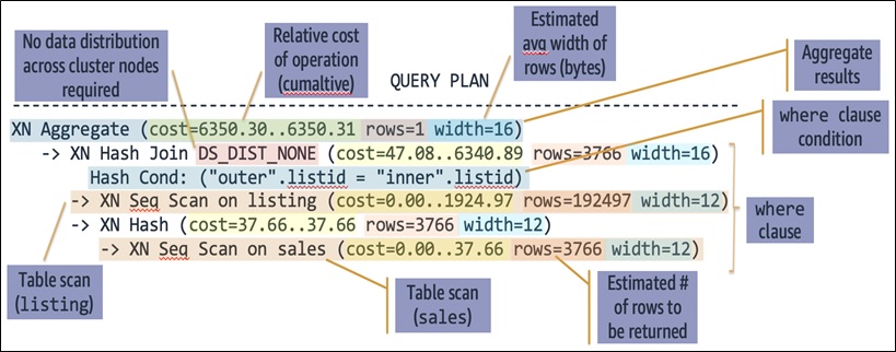
Figure 5 – Execution plan of the sample query.

Conclusion

By adopting the best practices that Onica has developed over years of using Amazon Redshift, you can improve the performance of your AWS data warehouse implementation.

Onica has completed multiple projects ranging from assessing the current state of an Amazon Redshift cluster to helping tune, optimize, and deploy new clusters.

.

.

Onica – APN Partner Spotlight

Onica is an APN Premier Consulting Partner and MSP. They provide cloud consulting, infrastructure, and managed services, ensuring customers have the best technical solutions to solve their business challenges and deliver value for their organization.

Contact Onica | Practice Overview

*Already worked with Onica? Rate this Partner

*To review an APN Partner, you must be an AWS customer that has worked with them directly on a project.