Using AtScale and Amazon Redshift to Build a Modern Analytics Program with a Lake House

By David P. Mariani, Chief Technology Officer – AtScale, Inc.
By Jahnavi Jilledumudi, Partner Solutions Architect – AWS

AtScale

There has been a lot of buzz about a new data architecture design pattern called a Lake House.

With a data lake or data warehouse, customers often had to compromise on several factors like performance, quality, or scale. A Lake House approach integrates a data lake with the data warehouse and all of the purpose-built stores so customers no longer have to take a one-size-fits-all approach and are able to select the storage that best suits their needs.

With customers storing data in multiple locations, there’s a need for a unified semantic layer on top of the data, so business intelligence (BI) analysts and data scientists have a single pane of glass through which they can access all of their data.

In this post, we’ll show how to take advantage of powerful and mature Amazon Web Services (AWS) technologies like Amazon Redshift, coupled with a semantic layer from AtScale, to deliver fast, agile, and analysis-ready data to business analysts and data scientists.

AtScale is an AWS Partner that delivers a universal semantic platform for BI and machine learning (ML) on Amazon Redshift and Amazon Simple Storage Service (Amazon S3).

Main Ingredients

The core components of a Lake House architecture include shared object storage, warehouse, shared data catalog, and access to multiple data processing engines.

AWS offerings in these areas include:

• Shared object storage: Amazon S3 is a durable and reliable storage service that can be used to back virtually any AWS service. It’s specifically designed to provide query-in-place functionality, allowing customers to run powerful analytics directly on data at rest in S3.
• Shared data warehouse: Amazon Redshift is a data warehouse in the cloud that lets you store, query, and combine exabytes of structured and semi-structured data in seconds.
• Shared data catalog: AWS provides several mechanisms for sharing data catalogs between processing services. For example, AWS Glue Data Catalog can maintain and expose a shared data catalog service that can be used and accessed by services like Amazon EMR and Amazon Redshift.
• Built-for-purpose data processing: With shared storage and a shared data catalog in place, AWS customers can seamlessly use processing services like Amazon EMR to do large-scale batch data processing, while also using Amazon Redshift Spectrum to execute analytic queries against the same base data.

Combining the components above with a business-friendly semantic layer delivers value by making data consumable by anyone.

In the world of data lakes and cloud data warehouses, combined with the rapid growth of self-service data analytics, there are some core requirements that a modern analytics platform must satisfy:

• First, these platforms must deliver a design experience that enables the creation of business-friendly data models directly on data stored in cloud storage platforms like Amazon S3.
• Next, a successful platform needs to enable an interactive, highly concurrent, query experience for business users and data scientists without requiring data movement off of the data lake.
• Finally, a modern platform for data lake intelligence needs to support a wide range of client access modes, including SQL, MDX (Multidimensional Expressions), DAX (Data Analysis Expressions), REST, and Python.

Along with core AWS services, AtScale delivers a platform that robustly satisfies all of these key requirements. AtScale enables a design experience directly on S3 data, while its autonomous data engineering feature leverages Amazon Redshift to deliver an interactive query experience.

AtScale’s open data interface allows tools like Tableau, Excel, Power BI, and Jupyter Notebooks to easily access and query data without requiring additional data transformation, data movement, or tool-specific extracts.

In the rest of this post, we’ll provide an end-to-end demonstration of how S3, Amazon Redshift, Amazon Redshift Spectrum, and AtScale provide a complete solution for cloud-based data lake house intelligence.

Use Case: Analyzing Amazon CloudFront Logs Using AtScale

For the purpose of this scenario, imagine there’s a need to allow business analysts and data scientists to easily interact with and analyze the performance of content delivered using Amazon CloudFront, a content delivery network (CDN).

For this example, we’ll create an external table using Amazon Redshift Spectrum, create a semantic layer using AtScale, and then query and optimize the underlying data and queries using Amazon Redshift.

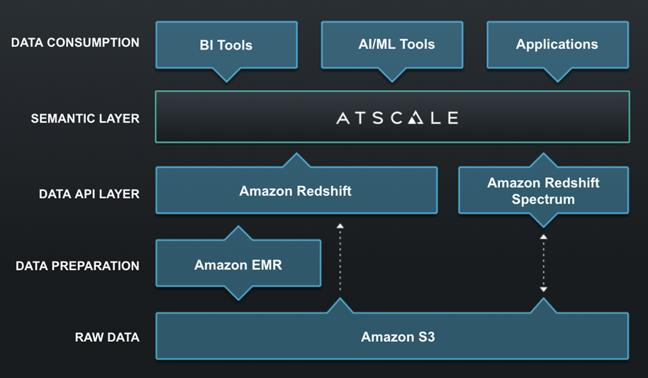
Figure 1 – AtScale semantic layer between your data warehouse and BI tool.

Now, let’s dive into the specific steps to realize this use case.

Step 1: Parse Raw CloudFront Logs and Create a Hive Data Set

The logs for Amazon CloudFront are stored on S3, and the first step to making them consumable is to use a batch processing system like Amazon EMR to prepare the data.

Given the volume of raw CDN data and the batch nature of data parsing required, this EMR processing step may be run on a daily or hourly basis, writing back row-level records back to S3.

The Hive DDL to create the table looks like:

CREATE EXTERNAL TABLE IF NOT EXISTS cloudfront_logs ( 
	DateObject Date, 
	Time STRING, 
	Location STRING, 
	Bytes INT, 
	RequestIP STRING, 
	Method STRING, 
	Host STRING, 
	Uri STRING, 
	Status INT, 
	Referrer STRING, 
	OS String, 
	Browser String, 
	BrowserVersion String 
)

The Hive code that parses the log files using the RegEx SerDe looks like this:

ROW FORMAT SERDE 'org.apache.hadoop.hive.serde2.RegexSerDe' 
WITH SERDEPROPERTIES ( 
  "input.regex" = "^(?!#)([^ ]+)\\s+([^ ]+)\\s+([^ ]+)\\s+([^ ]+)\\s+([^ ]+)\\s+([^ ]+)\\s+([^ ]+)\\s+([^ ]+)\\s+([^ ]+)\\s+([^ ]+)\\s+[^\(]+[\(]([^\;]+).*\%20([^\/]+)[\/](.*)$"
) LOCATION '${INPUT}/cloudfront/data/';

Step 2: Create an External Table Using Amazon Redshift Spectrum

Using the code above, a table called cloudfront_logs is created on S3, with a catalog structure registered in the shared AWS Glue Data Catalog.

Because of the shared nature of S3 storage and AWS Glue Data Catalog, this new table can be registered on Amazon Redshift using a feature called Spectrum.

Amazon Redshift Spectrum allows users to run SQL queries against raw data stored on S3. Essentially, this extends the analytic power of Amazon Redshift beyond data stored on local disks by enabling access to vast amounts of data on the S3 “data lake.”

The process of registering an external table using Amazon Redshift Spectrum is simple.

First, create an external schema that uses the shared data catalog:

create external schema spectrum from data catalog
database 'spectrumdb'
iam_role 'arn:aws:iam::123456789012:role/RedshiftSpectrumRole'
create external database if not exists;

Then, create an external table reference that points to the CloudFront data that was output from the EMR Hive process:

drop table spectrum.cloudfront;
create external table spectrum.cloudfront(
            DateObject CHARACTER VARYING(100), 
	Time CHARACTER VARYING(100), 
	Location CHARACTER VARYING(100), 
	Bytes INT, 
	RequestIP CHARACTER VARYING(100), 
	Method CHARACTER VARYING(100), 
	Host CHARACTER VARYING(100), 
	Uri CHARACTER VARYING(100), 
	Status INT, 
	Referrer CHARACTER VARYING(100), 
	OS CHARACTER VARYING(100), 
	Browser CHARACTER VARYING(100), 
	BrowserVersion CHARACTER VARYING(100) 
)
stored as parquet
location 's3://s3bucketname/parquet/cloudfront/';

To view the external Amazon Redshift Spectrum table definition and confirm its creation, you may query the SVV_EXTERNAL_COLUMNS system view within your Amazon Redshift database.

Step 3: Create an AtScale Semantic Model on the CloudFront Dataset

Once the CloudFront dataset in S3 has been registered within Amazon Redshift, it’s possible to start creating a semantic layer with AtScale using this data set as the core building block.

The screenshot below shows what the design experience in AtScale looks like when designing a semantic layer on top of data in Amazon Redshift and Amazon S3.

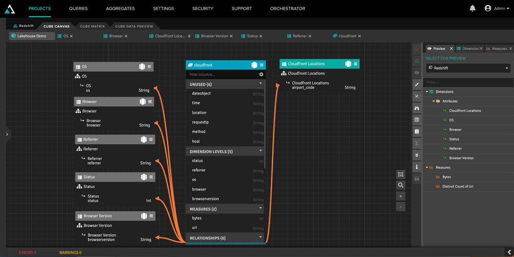
Figure 2 – Dimensional modeling in AtScale.

The screenshot above highlights several core capabilities that AtScale and AWS are able to support when used as an end-to-end data lake intelligence solution:

• The core fact table in this model, cloudfront, is available for modeling within AtScale. However, this “table” is simply an external reference (using Amazon Redshift Spectrum) to the raw data set residing in S3. This means AtScale model designers can create semantic layers directly on data in S3.
• Note that this model is able to blend raw data from S3 (the aforementioned cloudfront table) with data that already exists in Amazon Redshift tables. In this case, there’s a dimension (CloudFront Location) that is sourced from a table, cloudfront_location, that’s stored in an Amazon Redshift database.
• AtScale is able to build a traditional dimensional model (with measures, dimensions, and hierarchies) with a mix of underlying schema representations. For example, while the CloudFront Location dimension is modeled like a traditional dimension in a star schema, the browser and operating system (OS) dimensions are based directly off of the fact table, taking the form of a degenerate dimension.

This level of flexibility means that AtScale, Amazon Redshift, and Amazon S3 can be used together to support a broad range of raw data structures sourced from a data lake and/or a cloud data warehouse.

Step 4: Run Queries in Tableau, Excel, Power BI, and Jupyter Notebooks

Once created, the AtScale semantic layer can be exposed to virtually any data analytics tool that generates SQL, MDX, DAX, REST, or Python queries.

Let’s take a look at what the CloudFront model looks like when queried using Tableau.

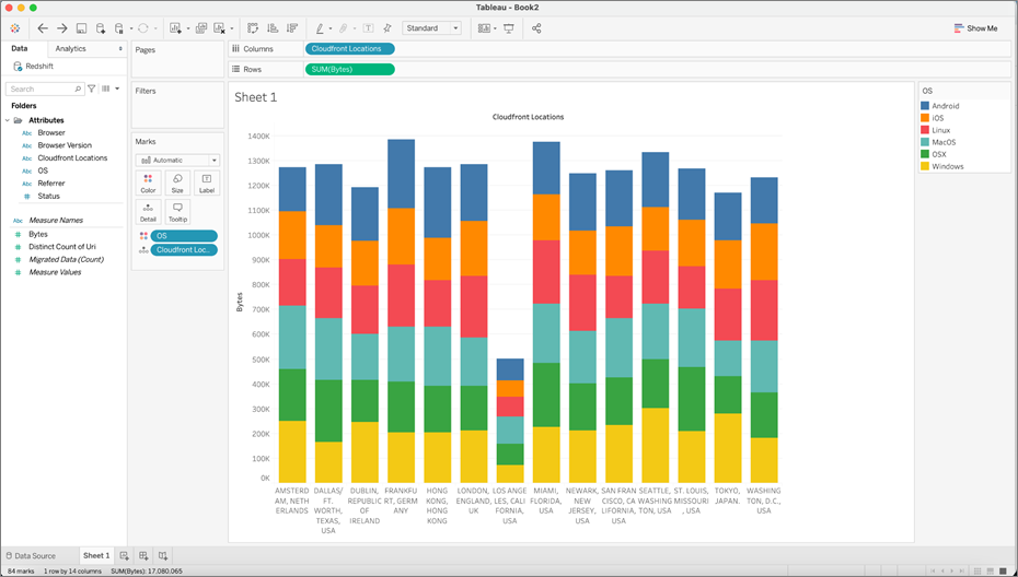
Figure 3 – Tableau report showing number of bytes by Location and Device Type/OS.

In this view, we are showing the total number of bytes distributed across CloudFront locations, and with the OS of the requestor highlighted by different colors. Note there are 255,475 bytes associated with Linux for CloudFront Locations in Miami, FL.

Looking at the query logs for this query in AtScale helps to better understand the mechanics of the system. First, the inbound query (the query from Tableau to AtScale) shows a very simple SELECT with a GROUP BY:

SELECT `Redshift`.`Cloudfront Locations` AS `cloudfront_locations`,
  `Redshift`.`OS` AS `os`,
 SUM(`Redshift`.`m_bytes_sum`) AS `sum_m_bytes_sum_ok`
FROM `redshift`.`redshift` `Redshift`
GROUP BY 1, 2

Upon receiving this query, AtScale uses its knowledge of the AtScale semantic model, along with the availability of data on the Amazon Redshift cluster, to construct an appropriate query to push down to Amazon Redshift, as show in the outbound query below:

SELECT
   t_25.cloudfront_locatio_gbakc3 AS cloudfront_locations,
   t_25.os_gbakc4 AS os,
   t_25.sum_m_bytes_sum_ok_gbakc5 AS sum_m_bytes_sum_ok
FROM
(
   SELECT
      cloudfront_locatio_t23.city_name AS cloudfront_locatio_gbakc3,
      cloudfront_t21.os AS os_gbakc4,
      CAST(SUM(cloudfront_t21.bytes) AS BIGINT) AS sum_m_bytes_sum_ok_gbakc5,
      cloudfront_locatio_t23.airport_code AS cloudfront_locatio_gbakc1,
      cloudfront_t21.os AS os_gbakc2
   FROM
      spectrum.cloudfront AS cloudfront_t21
   JOIN
      cloudfront_demo.cloudfront_locations AS cloudfront_locatio_t23
   ON
      SUBSTRING(location,1,3) = cloudfront_locatio_t23.airport_code
   WHERE
      true
   GROUP BY 1, 2, 4, 5
) AS t_25

Note the query above is able to access both the CloudFront data in S3 (by querying the previously created spectrum.cloudfront table) and join it with data stored as a native Amazon Redshift table: the cloudfront_location table.

Let’s take a look at a query using this same AtScale semantic model from Excel.

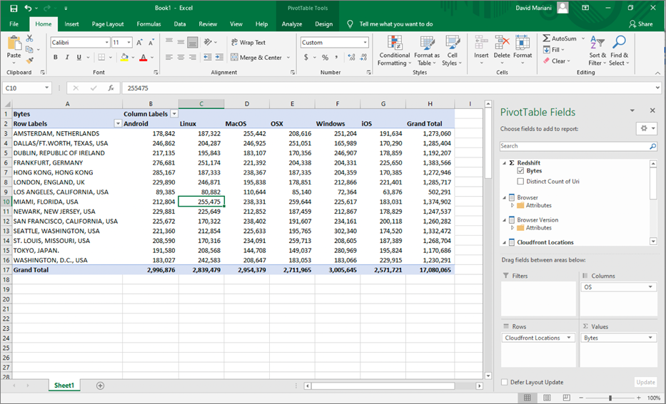
Figure 4 – Excel report showing the number of bytes by location and OS.

Note that even though the BI client in this case is different, the results are identical to the Tableau results: 255,475 bytes for Linux and Miami, FL. Also, note the inbound query for this result set was created in MDX instead of SQL.

SELECT 
NON EMPTY Hierarchize({DrilldownLevel({[OS].[OS].[All]},,,INCLUDE_CALC_MEMBERS)}) DIMENSION PROPERTIES PARENT_UNIQUE_NAME,HIERARCHY_UNIQUE_NAME 
ON COLUMNS , 
NON EMPTY Hierarchize({DrilldownLevel({[Cloudfront Locations].[Cloudfront Locations].[All]},,,INCLUDE_CALC_MEMBERS)}) DIMENSION PROPERTIES PARENT_UNIQUE_NAME,HIERARCHY_UNIQUE_NAME 
ON ROWS  
FROM [Redshift] 
WHERE ([Measures].[m_bytes_sum]) 
CELL PROPERTIES VALUE, FORMAT_STRING, LANGUAGE, BACK_COLOR, FORE_COLOR, FONT_FLAGS

Just like Tableau and Excel, the AtScale semantic layer also delivers a live connection to Power BI using the DAX protocol.

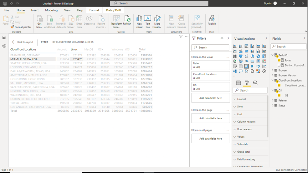
Figure 5 – Power BI report showing bytes by location and OS.

Again, the answers are the same regardless of the client tool. Moreover, in Power BI, if you select the “Model” view, you can see the same model we created in AtScale Design Center.

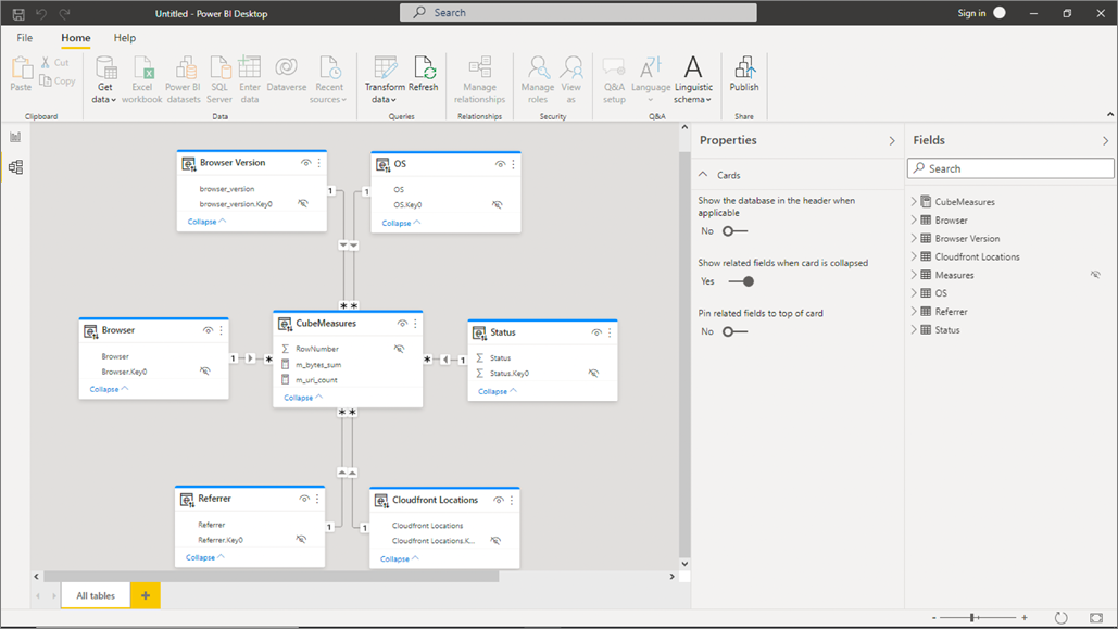
Figure 6 – View of the data model in Power BI.

There’s no need to reinvent the wheel—the AtScale semantic model is automatically inherited by Power BI using its live DAX connection. This ensures consistency and reduces time-consuming and redundant data engineering work.

The AtScale semantic layer also works for data scientists (as you can see below) with Amazon SageMaker using a Jupyter Notebook connected through Python.

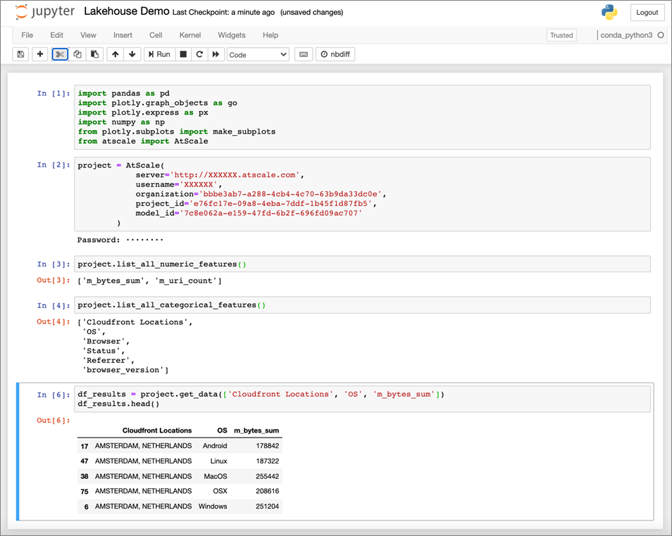
Figure 7 – Accessing AtScale model from Amazon SageMaker using Jupyter Notebook.

AtScale Query Acceleration on Amazon Redshift

As this scenario highlights, AtScale’s semantic layer—with its support for SQL, MDX, DAX, REST, and Python clients—is able to act as a single and consistent interface for business intelligence and data science.

This capability alone is of great value to enterprises trying to bridge the gap between their big data platforms and analytics consumers.

In order to enable interactive query performance on the largest datasets, AtScale constantly monitors end user query patterns and determines if the creation of an aggregate table would more efficiently satisfy similar versions of the same query.

The collection of aggregate tables that are created (and maintained) by AtScale for a specific model are called Acceleration Structures. The resulting aggregate tables are stored directly on the host data platform; in this example, AtScale aggregates are stored on Amazon Redshift.

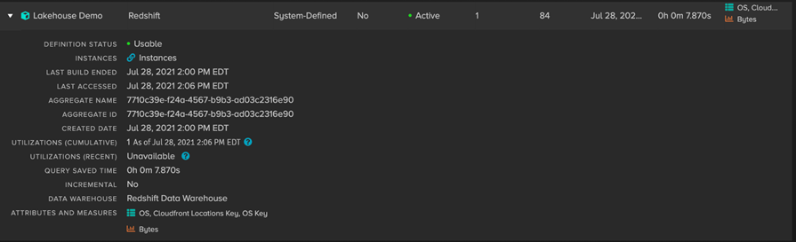
Figure 8 – AtScale aggregates on Amazon Redshift data warehouse.

This aggregate was created in response to the original Tableau query that requested the sum of Bytes grouped by OS and Location. This means that for the MDX query from AtScale, the query can be satisfied by an AtScale managed aggregate table in Amazon Redshift and not the raw data in Spectrum.

The outbound query to satisfy the Excel-derived MDX query is shown below:

SELECT
   cloudfront_locatio_t14.city_name AS c0,
   cloudfront_locatio_t14.airport_code AS c1s0,
   CAST(SUM(as_agg_77f3327a_no_t13.m_bytes_sum_c2) AS BIGINT) AS c2
FROM
   atscale.as_agg_77f3327a_none AS as_agg_77f3327a_no_t13
JOIN
   cloudfront_demo.cloudfront_locations AS cloudfront_locatio_t14
ON
   as_agg_77f3327a_no_t13.key_c1 = cloudfront_locatio_t14.airport_code
WHERE
   true
GROUP BY 1, 2
ORDER BY 1 ASC NULLS FIRST

Although this query hit the aggregate table (and as a result was faster than a query against the raw data), the results and user experience were consistent for the end user.

Conclusion

In this post, we have shown how AtScale complements Lake House architecture by adding a meaningful semantic layer, creating a data model and defining the measures and dimensions in the data, shielding the analyst from where data is stored within the lake house, and delivering consistent and results regardless of the BI tool used to query the data.

We have also seen how AtScale can increase the performance of queries by automatically creating aggregate tables based on observing query patterns.

With AtScale and AWS, Lake House intelligence is possible without compromises. The Lake House architecture provides the ability to store, access, and analyze vast amounts of data. By combining these technologies with the AtScale semantic layer, organizations can deploy a modern architecture that drives business agility.

AtScale and AWS can help service the needs of business users and data scientists alike while providing speed, security, governance, and flexibility.

.

.

AtScale – AWS Partner Spotlight

AtScale is an AWS Partner that delivers a universal semantic platform for business intelligence and machine learning on Amazon Redshift and Amazon S3.

Contact AtScale | Partner Overview

*Already worked with AtScale? Rate the Partner

*To review an AWS Partner, you must be a customer that has worked with them directly on a project.