Using Databricks SQL on Photon to Power Your AWS Lake House

By Volker Tjaden, Partner Solutions Architect and APN Ambassador – Databricks

Databricks, an AWS Partner with the Data and Analytics Competency, recently released Databricks SQL, a dedicated workspace for data analysts. It comprises a native SQL editor, drag-and-drop dashboards, and built-in connectors for all major business intelligence (BI) tools as well as Photon, a next-generation query engine compatible with the Spark SQL API.

In combination, these innovations complete the Databricks Lakehouse on AWS, which enables BI and SQL analytics use cases directly on a customer’s Amazon Simple Storage Service (Amazon S3) data lake.

In addition to realizing cost savings, the customer thereby avoids data duplication and can run BI queries on the entire dataset without having to rely on data extracts.

In this post, I will introduce you to the technical capabilities of the new features and walk you through two examples: ingesting, querying, and visualizing AWS CloudTrail log data, and building near real-time dashboards on data coming from Amazon Kinesis.

As a Partner Solutions Architect at Databricks, I partner with teams from Amazon Web Services (AWS) to help them use the Databricks platform to jointly realize Lakehouse deployments integrated into customers’ AWS accounts.

I have been an APN Ambassador since 2021. APN Ambassadors work closely with AWS Solutions Architects to migrate, design, implement, and monitor AWS workloads.

The Lake House Paradigm

The Lake House paradigm is an architectural pattern for data platforms that recently emerged and has since won endorsements from various vendors and sub-disciplines in the data domain, including Bill Inmon who is one of the pioneers of data warehousing.

The central proposition of the Lake House is that the elasticity and scalability of the public cloud enable the creation of a single enterprise-wide data platform for storing, refining, and enriching all relevant datasets. This can simultaneously feed BI as well as data science and machine learning (ML) use cases.

A data pipeline built for a particular use case can thus be structured in such a way to allow for easy reuse in adjacent use cases.

Think, for example, of a company that wants to build artificial intelligence-driven personalization features for their users. The data integration work involved in building the 360-degree data view of customers that’s needed to feed those algorithms typically contains a lot of relevant insights into user behavior that would have been previously unattainable.

On a technological level, the central underpinning of a Lake House is a data layer that can implement the structures and management features known from data warehousing directly on low-cost data lake data storage such as Amazon S3 (hence the term Lake House).

This layer ties into a high-performance execution engine that can seamlessly scale to process the petabyte-scale datasets required for large-scale ML applications, while simultaneously satisfying the latency and concurrency requirements of BI dashboarding applications.

The Databricks Lakehouse is built on Delta Lake and Apache Spark. Spark has long been known as the most powerful tool for building large-scale data engineering and ML applications. However, for analysts wanting to standardize on Databricks for explorative SQL-based work, the experience was far from optimal due to the lack of a native work environment, a performance overhead when querying smaller datasets, and poor support for connecting with BI tools.

To provide those user personas with a first-class experience, Databricks recently released Databricks SQL, a dedicated workspace for data analysts.

Databricks SQL

Databricks SQL allows Databricks customers to perform BI and SQL workloads on their AWS Lake House. The new service consists of four main components.

SQL-Native Workspace

The new workspace is a separate environment for data analysts that equips them with familiar tooling, such as a SQL query editor with auto-completion, interactive schema exploration, and the ability to schedule queries for regular refreshes. The results of the queries can be visualized in drag-and-drop dashboards.

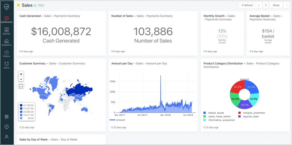
Figure 1 – Interactive dashboards in Databricks SQL.

Built-In Connectors to Existing BI Tools

Databricks SQL includes built-in connectors to major BI tools such as Tableau, Power BI, and Qlik. The connectors provide significant performance benefits in the client-to-endpoint communication over connecting by plain JDBC/ODBC.

They can also use a capability called Cloud Fetch that allows parallelizing data retrieval by first offloading the query results to cloud storage.

SQL Endpoints

In order to satisfy the concurrency and latency requirements of BI workloads, Databricks SQL workloads are run on optimized Databricks clusters called SQL endpoints.

These run on instances from the i3-family to leverage caching on the cluster nodes. They also introduce a new form of auto-scaling which responds to increased query workloads by adding one or more clusters and load balancing between the clusters.

Further performance-enhancing features are the use of queuing to prioritize high-priority low-latency queries, async and parallel IO to speed up performance when querying small files, and of course the Photon engine.

Governance and Administration Features

SQL data access controls introduce many of the fine-grained permissions available in data warehouses to the data lake. Additionally, the query history allows auditing along with providing performance statistics to allow for debugging and performance tuning.

For a more in-depth description of the individual components, check out the Databricks blog.

Photon

Photon is a native vectorized engine developed in C++ to take advantage of the latest vectorized query processing to capitalize on data- and instruction-level parallelism in CPUs.

Photon is ultimately designed to accelerate all workloads, but the initial focus is on running SQL workloads faster. There are two ways a customer can use Photon on Databricks: 1) As the default query engine on Databricks SQL, and 2) as part of a new high-performance runtime on Databricks clusters.

Figure 2 – Performance comparisons for the Photon engine against previous Databricks runtimes relative to version 2.1.

The preceding graph plots relative performance for different versions of the Databricks Runtime on the Power Test from the 1TB TPC-DS benchmark. The step change in performance introduced by Photon is easily visible. Performance was increasing steadily over time, but switching to Photon introduces a 2x speedup compared to the Databricks Runtime 8.0.

Internally, Photon integrates in and with Databricks Runtime and Spark, which means that no code changes are required to use Photon. At the time of writing, Photon did not yet support all features that Spark does, so a single query may end running partially in Photon and partially in Spark.

During the preview, customers observed 2-4x average speedups using Photon on SQL workloads. This included large-scale SQL-based extract, transform, load (ETL), time-series analysis on Internet of Things (IoT) data, data privacy and compliance on petabyte-scale datasets, and loading data into Delta and Parquet through Photon’s vectorized I/O.

On the Databricks blog, the story Announcing Photon Public Preview: The Next Generation Query Engine on the Databricks gives a more thorough introduction and deep dive into the integration with Spark’s Catalyst optimizer.

In the remainder of this post, I’ll walk you through two example applications for using Photon and Databricks SQL with Databricks running on AWS. Readers who want to follow along may find all notebooks available for download in this Github repository.

Real-Time Dashboards Using IoT Data from Amazon Kinesis

The management and analysis of real-time IoT device data from Amazon Kinesis is the first example application for Databricks SQL and Photon that I want to explore.

In the context of streaming, analytics applications have traditionally faced the challenge of running real-time analytics at sub-second latencies on the data as it’s coming in, and consolidating the individual messages into large tables stored in Amazon S3 to run queries on the entire history.

Initial approaches to simultaneously fulfilling these demands have relied on an AWS Lambda architecture that separates the data into a speed layer for the low-latency queries and a batch layer for offline storage and big data analytics. This, however, has come with its own set of challenges—having to build business logic separately between speed and batch layers, and ensuring the state between the two does not diverge.

The combination of Delta Lake and Spark Structured Streaming demonstrated in this example takes a different approach. Here, we define streaming queries on the data as it’s coming in while simultaneously writing the data out to Delta Lake tables which themselves can serve as upstream streaming sources for queries.

This effectively reunifies batch and streaming analytics while relying on one single set of APIs for writing the queries.

To follow along with this walkthrough, use the Databricks notebooks in the folder kinesis_iot_data. The main notebook to follow is main_notebook.dbc. You need to provide the name of an S3 bucket and the name of an Amazon Kinesis data stream to use in iot_init.dbc.

The notebook gen_iot_stream.dbc generates the simulated IoT data for the main notebook and posts the data to Kinesis. You need to run the notebook on a Databricks cluster with an instance profile that has permissions to access the S3 bucket and Kinesis.

If you want to register the tables in an AWS Glue database, you will need additional permissions for AWS Glue.

Step 1: Set Up a Stream for Raw Data and Write to Bronze-Table

After setting up the static metadata tables, as well as the Kinesis stream with the simulated device data, we configure a Spark streaming job to read the data from Kinesis.

The raw messages as they are fetched from Kinesis are schematized in such a way that the message is contained in a serialized form in the data field (see Amazon Kinesis | Databricks on AWS), which we need to explicitly cast to string format for it to be readable.

We also directly apply the JSON schema of the messages to make each field available as a separate column in the resulting dataframe.

from pyspark.sql.types import *
from pyspark.sql.functions import col, from_json

sensor_schema = StructType()\
  .add('timestamp',TimestampType()) \
  .add('deviceId',IntegerType()) \
  .add('temperature',DoubleType())

sensor_readings = (spark
  .readStream
  .format("kinesis")
  .option("streamName", my_stream_name)
  .option("initialPosition", "latest")
  .option("region", kinesisRegion)
  .load()
  .withColumn('payload',col("data").cast(StringType()))
  .withColumn('json',from_json(col('payload'),sensor_schema))
  )

sensor_readings.createOrReplaceTempView('sensor_readings')

After registering the dataframe as a temporary view, it can be referenced in SQL queries whose results are updated and visualized live inside the Databricks notebook.

%sql

select json.deviceId, min(json.temperature) as min, max(json.temperature) as max, avg(json.temperature) as mean
from sensor_readings
group by deviceId
order by deviceId asc

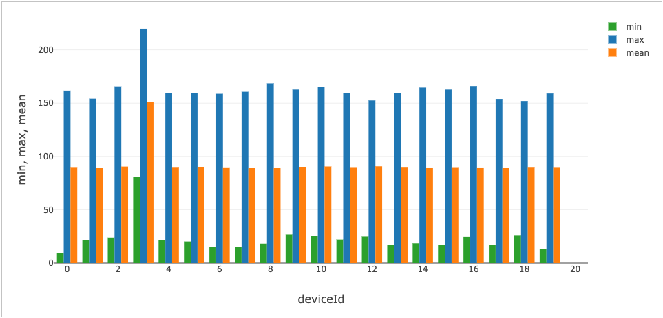
Figure 3 – Summary statistics on the simulated device data reveal sensor 3 as a potential outlier.

A brief inspection of the data reveals one device to be sending back much higher temperature readings than the rest of the sensors. We’ll momentarily join the data with additional information on the sensors to determine whether this hints at a problem.

Before that, however, we’ll write the data out to a “bronze-level” Delta Lake table while also quarantining sensor readings without temperature to a separate bad records table. This way, the error readings don’t pollute downstream tables but are still available for later analysis.

def to_bronze_table(df,epoch_id):
  df.persist()
  # Write correct data to bronze path
  (df
   .filter('json.temperature is not null')
   .select('json.*')
   .write
   .mode("append")
   .format('delta')
   .save(bronze_path)
  )
  
  # Write erroneous data to separate delta table as error queue
  (df
   .filter('json.temperature is null')
   .write
   .mode("append")
   .format('delta')
   .save(bad_records_path)
  )
  
  df.unpersist()

sensor_readings.writeStream.foreachBatch(to_bronze_table).start()

Step 2: Create Silver Table with Added Metadata

As a next step, we create a “silver-level” table in which the data is enriched with additional information on the individual sensors, as well as the plant locations we’ll use in the final dashboard. In addition, we add in extra columns to flag readings where the temperature falls outside of defined specifications for the sensor.

In the following streaming query, we treat our previously defined bronze table as a streaming source such that any additional data in the bronze table is automatically read, joined, transformed, and then added to the silver table. The use of checkpointing ensures exactly once processing in the event of failure.

from pyspark.sql.functions import col

locations = spark.read.table('locations')
sensors = spark.read.table('sensors')

silver_stream = (spark.readStream
                 .format('Delta')
                 .load(bronze_path)
                 .join(sensors, on=['deviceId'])
                 .join(locations, on=['l_id'])
                 .withColumn('Temp_high_alert', col('temperature') > col('max_accept_temp'))
                 .withColumn('Temp_low_alert', col('temperature') < col('min_accept_temp'))
                 .writeStream
                 .format("delta")
                 .option("checkpointLocation",checkpointPathSilver)
                 .outputMode("append")
                 .queryName('silver_query')
                 .table('iot_silver')
                )

Step 3: Create Gold Table to Feed Monitoring Dashboard

Finally, we use aggregation on time-based window functions to construct a gold-level table on which to build an alerting dashboard. Instead of flagging every reading outside of the specified bounds, we want to focus on sensors with a large share of extreme readings per minute.

from pyspark.sql.functions import window, avg, count, sum

gold_stream = (spark.readStream
               .format('delta')
               .load(silver_path)
               .withWatermark('timestamp','1 minutes')
               .withColumn('in_alert',(col('Temp_high_alert') == True) | (col('Temp_low_alert') == True))
               .withColumn('in_alert',col('in_alert').cast(IntegerType()))
               .groupBy(window('timestamp','60 seconds'),'deviceId','name','latitude','longitude')
               .agg(avg('temperature').alias('mean_temp'),
                    count('*').alias('event_no'),
                    sum('in_alert').alias('alert_no')
                   )
               .withColumn('alert_share',col('alert_no')/col('event_no'))
               .select(col('window.start').alias('start'), 
                       col('window.end').alias('end'), 'deviceId','name','latitude','longitude',
                       'mean_temp', 'event_no', 'alert_no', 'alert_share')
               .writeStream
               .option("checkpointLocation",checkpointPathGold)
               .outputMode("append")
               .queryName('gold_query')
               .table('iot_gold')
              )

Step 4: Build a Monitoring Dashboard on Databricks SQL

In a final step, we head over to the SQL console to define queries on which to build visualizations for our alerting dashboard. The below example shows our three simulated German plant locations with green and red dots displayed on a map to provide a high-level overview of potential problems per location.

We can then specify a plant and drill down for further analysis on a per-sensor level. The dashboard is scheduled to automatically refresh every minute to allow for fast response times to address emerging problems and malfunctions.

After you have finished building the dashboard, you can run notebook cleanup_iot.dbr to delete all resources that were created while following along.

Figure 4 – Monitoring dashboard aggregates status per location on a map. A red dot per location indicates a problem that we can drill down on in the right tables.

Building a Dashboard on AWS CloudTrail Logs

Another good example is the ingestion of AWS CloudTrail logs and the creation of a monitoring dashboard on top of those data.

AWS CloudTrail by default saves log files in a dedicated S3 bucket. By ingesting the files into Delta Lake, one can integrate them with other cybersecurity data we are monitoring in the company to create a comprehensive, near-real time view on any potential threat. Check out this resource to learn more about how Databricks is used for cybersecurity analytics.

After some ETL on the data, we can build a visualization of the log events without having to copy them into another specialized storage backend.

To follow along with this walkthrough, use the Databricks notebook in the folder cloud_trail. The notebook to follow is main_notebook.dbc.

You will need to provide the name of an S3 bucket to store the CloudTrail logs and one to store the ingested data in a Delta Lake table. You should run the notebook on a Databricks cluster with an instance profile that has sufficient permissions for accessing the S3 buckets.

Step 1: Set Up CloudTrail and Make the S3 Bucket Accessible in the Databricks Workspace

AWS CloudTrail saves logs as JSON text files in compressed gzip format (*.json.gzip), the location of which depends on the configuration of the trail. More information is available in the AWS CloudTrail User Guide:

If CloudTrail is not already in use in the AWS account, enable CloudTrail from the AWS Management Console. For more information, see Creating a Trail in the user guide.

After locating the destination S3 bucket where CloudTrail saves the logs, you need to make the logs accessible from within a Databricks workspace. The best practice for securely accessing S3 buckets from a Databricks cluster is the use of instance profiles; see Secure access to S3 buckets using instance profiles | Databricks on AWS.

In case Log-file SSE-KMS encryption is enabled for the S3 bucket, you will also need to add the instance profile as a key user for the AWS Key Management Services (AWS KMS) key and set encryption properties for the Databricks cluster. To learn more, see Amazon S3 | Databricks on AWS.

Step 2: Ingest Data into Delta Lake Using Auto Loader

The Databricks notebook for this step is accessible for download.

For ingesting data that continuously arrives in an S3 bucket into a Delta Lake table, Databricks provides a useful feature called Auto Loader.

input_path = 's3:/<CLOUTDTRAIL-BUCKET-NAME>/AWSLogs/<AWS-ACC-NO>/CloudTrail/*/*/*/*'
output_path = 's3://<YOUR-BUCKET-NAME>/cloudtrail/delta/'
schema = cloudTrailSchema
checkpoint_path = 's3://<YOUR-BUCKET-NAME>/cloudtrail/checkpoints/'


df_log = (spark
          .readStream
          .format('cloudFiles')
          .option('cloudFiles.useNotifications','true')
          .option('cloudFiles.format','json')
          .schema(cloudTrailSchema)
          .load(input_path)
          .select(explode('records').alias('record'))
          .select(
           unix_timestamp('record.eventTime',"yyyy-MM-dd'T'HH:mm:ss'Z'").cast(TimestampType()).alias('timestamp'),
                'record.*')
         )

(df_log
 .writeStream
 .format('delta')
 .option('checkpointLocation',checkpoint_path)
 .trigger(processingTime='10 seconds')
 .start(output_path)
)

In the above example, substitute in the name of the S3 bucket we located in Step 1, as well as your AWS account number. The four wildcards at the end of the input path mean we’ll be ingesting data from all regions as well as the entire history of log data. By specifying values for any of the wildcards, you can limited the dataset to either a specific region or time.

Auto Loader provides a Structured Streaming source called cloudFiles. By providing the JSON-schema for the CloudTrail log data and calling explode() on the individual records, we additionally transform the nested data to a tabular format for easier querying later on.

Next, we register the resulting table in either the Databricks or the Glue metastore so we can start querying it:

%sql
CREATE DATABASE IF NOT EXISTS cloudtrail_blog;
USE cloudtrail_blog;

CREATE TABLE logdata
USING DELTA
LOCATION 's3://<YOUR-OUTPUT-BUCKET-NAME>/cloudtrail/delta/'

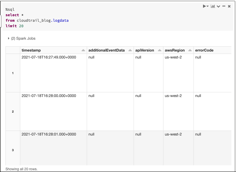
Figure 5 – Exploring the CloudTrail log data from within a Databricks notebook.

Finally, to obtain optimal latencies for our dashboard queries, we’ll run an OPTIMIZE command on the table to compact the underlying Parquet files into optimal sizes. Z-Ordering the data on timestamp will further speed up queries that filter data along the time dimension, as this changes the data layout to reduce the amount of data that needs to be read in those queries.

%sql
OPTIMIZE cloudtrail_blog.logdata ZORDER BY (timestamp)

Step 3: Build a Monitoring Dashboard on Databricks SQL

Finally, we switch to the Databricks SQL user interface where we can use SQL to further explore the CloudTrail log data and queries on which to build visualizations.

When a query is ready and a visualization has been defined on top, those can be added as widgets to dashboards for which we can define automatic update schedules for an always up-to-date view on our data.

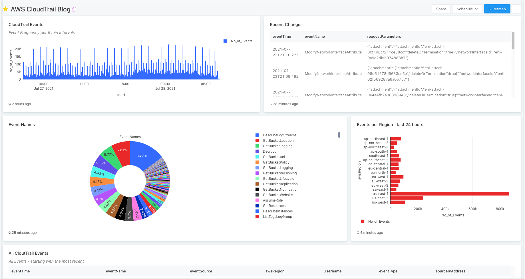
Figure 6 – Databricks SQL dashboard built on top of the CloudTrail log data.

Conclusion

In this post, I walked you through Databricks SQL and Photon, and explored two recent additions to the capabilities of the Databricks Lakehouse Platform on AWS.

I also demonstrated ingestion and analysis of real-time IoT data from Amazon Kinesis as well AWS CloudTrail log analytics as two example applications for those technologies.

If you want to learn more about the Databricks platform, see the Databricks website.

The content and opinions in this blog are those of the third-party author and AWS is not responsible for the content or accuracy of this post.

.

.

Databricks – AWS Partner Spotlight

Databricks is an AWS AWS Competency Partner that unifies all your data sources into a simple, open, and collaborative foundation of your Lake House.

Contact Databricks | Partner Overview | AWS Marketplace

*Already worked with Databricks? Rate the Partner

*To review an AWS Partner, you must be a customer that has worked with them directly on a project.