Get started with data integration from Amazon S3 to Amazon Redshift using AWS Glue interactive sessions

Organizations are placing a high priority on data integration, especially to support analytics, machine learning (ML), business intelligence (BI), and application development initiatives. Data is growing exponentially and is generated by increasingly diverse data sources. Data integration becomes challenging when processing data at scale and the inherent heavy lifting associated with infrastructure required to manage it. This is one of the key reasons why organizations are constantly looking for easy-to-use and low maintenance data integration solutions to move data from one location to another or to consolidate their business data from several sources into a centralized location to make strategic business decisions.

Most organizations use Spark for their big data processing needs. If you’re looking to simplify data integration, and don’t want the hassle of spinning up servers, managing resources, or setting up Spark clusters, we have the solution for you.

AWS Glue is a serverless data integration service that makes it easy to discover, prepare, and combine data for analytics, ML, and application development. AWS Glue provides both visual and code-based interfaces to make data integration simple and accessible for everyone.

If you prefer a code-based experience and want to interactively author data integration jobs, we recommend interactive sessions. Interactive sessions is a recently launched AWS Glue feature that allows you to interactively develop AWS Glue processes, run and test each step, and view the results.

There are different options to use interactive sessions. You can create and work with interactive sessions through the AWS Command Line Interface (AWS CLI) and API. You can also use Jupyter-compatible notebooks to visually author and test your notebook scripts. Interactive sessions provide a Jupyter kernel that integrates almost anywhere that Jupyter does, including integrating with IDEs such as PyCharm, IntelliJ, and Visual Studio Code. This enables you to author code in your local environment and run it seamlessly on the interactive session backend. You can also start a notebook through AWS Glue Studio; all the configuration steps are done for you so that you can explore your data and start developing your job script after only a few seconds. When the code is ready, you can configure, schedule, and monitor job notebooks as AWS Glue jobs.

If you haven’t tried AWS Glue interactive sessions before, this post is highly recommended. We work through a simple scenario where you might need to incrementally load data from Amazon Simple Storage Service (Amazon S3) into Amazon Redshift or transform and enrich your data before loading into Amazon Redshift. In this post, we use interactive sessions within an AWS Glue Studio notebook to load the NYC Taxi dataset into an Amazon Redshift Serverless cluster, query the loaded dataset, save our Jupyter notebook as a job, and schedule it to run using a cron expression. Let’s get started.

Solution overview

We walk you through the following steps:

1. Set up an AWS Glue Jupyter notebook with interactive sessions.
2. Use notebook’s magics, including AWS Glue connection and bookmarks.
3. Read data from Amazon S3, and transform and load it into Redshift Serverless.
4. Save the notebook as an AWS Glue job and schedule it to run.

Prerequisites

For this walkthrough, we must complete the following prerequisites:

1. Upload Yellow Taxi Trip Records data and the taxi zone lookup table datasets into Amazon S3. Steps to do that are listed in the next section.
2. Prepare the necessary AWS Identity and Access Management (IAM) policies and roles to work with AWS Glue Studio Jupyter notebooks, interactive sessions, and AWS Glue.
3. Create the AWS Glue connection for Redshift Serverless.

Upload datasets into Amazon S3

Download Yellow Taxi Trip Records data and taxi zone lookup table data to your local environment. For this post, we download the January 2022 data for yellow taxi trip records data in Parquet format. The taxi zone lookup data is in CSV format. You can also download the data dictionary for the trip record dataset.

1. On the Amazon S3 console, create a bucket called my-first-aws-glue-is-project-<random number> in the us-east-1 Region to store the data.S3 bucket names must be unique across all AWS accounts in all the Regions.
2. Create folders nyc_yellow_taxi and taxi_zone_lookup in the bucket you just created and upload the files you downloaded.
   Your folder structures should look like the following screenshots.

Prepare IAM policies and role

Let’s prepare the necessary IAM policies and role to work with AWS Glue Studio Jupyter notebooks and interactive sessions. To get started with notebooks in AWS Glue Studio, refer to Getting started with notebooks in AWS Glue Studio.

Create IAM policies for the AWS Glue notebook role

Create the policy AWSGlueInteractiveSessionPassRolePolicy with the following permissions:

{
    "Version": "2012-10-17",
    "Statement": [
        {
        "Effect": "Allow",
        "Action": "iam:PassRole",
        "Resource":"arn:aws:iam::<AWS account ID>:role/AWSGlueServiceRole-GlueIS"
        }
    ]
}

This policy allows the AWS Glue notebook role to pass to interactive sessions so that the same role can be used in both places. Note that AWSGlueServiceRole-GlueIS is the role that we create for the AWS Glue Studio Jupyter notebook in a later step. Next, create the policy AmazonS3Access-MyFirstGlueISProject with the following permissions:

{
    "Version": "2012-10-17",
    "Statement": [
        {
            "Effect": "Allow",
            "Action": [
                "s3:GetObject",
                "s3:ListBucket"
            ],
            "Resource": [
                "arn:aws:s3:::<your s3 bucket name>",
                "arn:aws:s3:::<your s3 bucket name>/*"
            ]
        }
    ]
}

This policy allows the AWS Glue notebook role to access data in the S3 bucket.

Create an IAM role for the AWS Glue notebook

Create a new AWS Glue role called AWSGlueServiceRole-GlueIS with the following policies attached to it:

• AWSGlueServiceRole
• AwsGlueSessionUserRestrictedNotebookPolicy
• AWSGlueInteractiveSessionPassRolePolicy
• AmazonS3Access-MyFirstGlueISProject

Create the AWS Glue connection for Redshift Serverless

Now we’re ready to configure a Redshift Serverless security group to connect with AWS Glue components.

1. On the Redshift Serverless console, open the workgroup you’re using.
   You can find all the namespaces and workgroups on the Redshift Serverless dashboard.
2. Under Data access, choose Network and security.
3. Choose the link for the Redshift Serverless VPC security group.You’re redirected to the Amazon Elastic Compute Cloud (Amazon EC2) console.
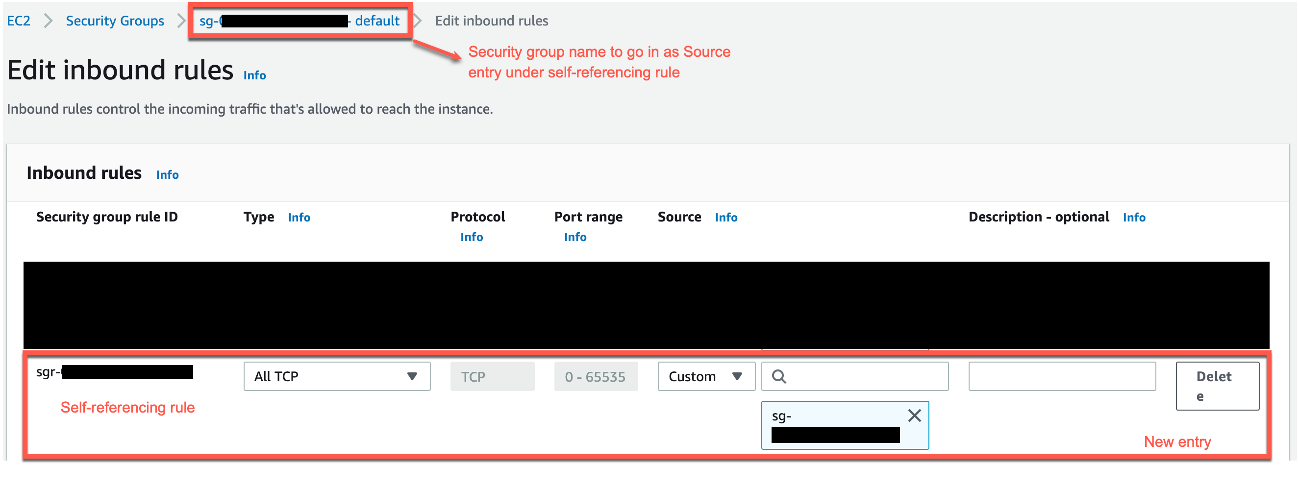
4. In the Redshift Serverless security group details, under Inbound rules, choose Edit inbound rules.
5. Add a self-referencing rule to allow AWS Glue components to communicate:
   1. For Type, choose All TCP.
   2. For Protocol, choose TCP.
   3. For Port range, include all ports.
   4. For Source, use the same security group as the group ID.
      
6. Similarly, add the following outbound rules:
   1. A self-referencing rule with Type as All TCP, Protocol as TCP, Port range including all ports, and Destination as the same security group as the group ID.
   2. An HTTPS rule for Amazon S3 access. The s3-prefix-list-id value is required in the security group rule to allow traffic from the VPC to the Amazon S3 VPC endpoint.
      

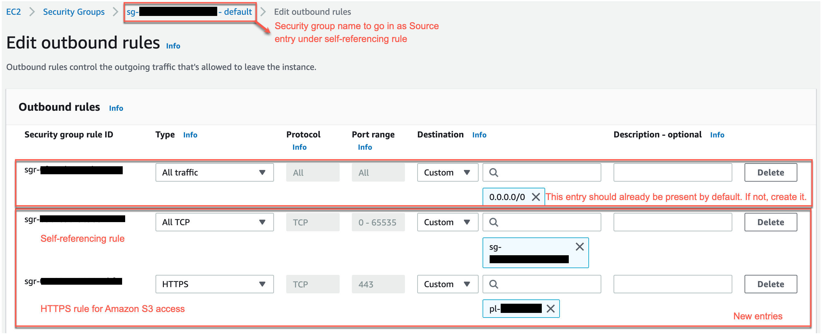
If you don’t have an Amazon S3 VPC endpoint, you can create one on the Amazon Virtual Private Cloud (Amazon VPC) console.

You can check the value for s3-prefix-list-id on the Managed prefix lists page on the Amazon VPC console.

Next, go to the Connectors page on AWS Glue Studio and create a new JDBC connection called redshiftServerless to your Redshift Serverless cluster (unless one already exists). You can find the Redshift Serverless endpoint details under your workgroup’s General Information section. The connection setting looks like the following screenshot.

Write interactive code on an AWS Glue Studio Jupyter notebook powered by interactive sessions

Now you can get started with writing interactive code using AWS Glue Studio Jupyter notebook powered by interactive sessions. Note that it’s a good practice to keep saving the notebook at regular intervals while you work through it.

1. On the AWS Glue Studio console, create a new job.
2. Select Jupyter Notebook and select Create a new notebook from scratch.
3. Choose Create.
   
4. For Job name, enter a name (for example, myFirstGlueISProject).
5. For IAM Role, choose the role you created (AWSGlueServiceRole-GlueIS).
6. Choose Start notebook job.
   After the notebook is initialized, you can see some of the available magics and a cell with boilerplate code. To view all the magics of interactive sessions, run %help in a cell to print a full list. With the exception of %%sql, running a cell of only magics doesn’t start a session, but sets the configuration for the session that starts when you run your first cell of code.For this post, we configure AWS Glue with version 3.0, three G.1X workers, idle timeout, and an Amazon Redshift connection with the help of available magics.
7. Let’s enter the following magics into our first cell and run it:

   %glue_version 3.0
   %number_of_workers 3
   %worker_type G.1X
   %idle_timeout 60
   %connections redshiftServerless

   We get the following response:

   Welcome to the Glue Interactive Sessions Kernel
   For more information on available magic commands, please type %help in any new cell.
   
   Please view our Getting Started page to access the most up-to-date information on the Interactive Sessions kernel: https://docs.aws.amazon.com/glue/latest/dg/interactive-sessions.html
   Installed kernel version: 0.35 
   Setting Glue version to: 3.0
   Previous number of workers: 5
   Setting new number of workers to: 3
   Previous worker type: G.1X
   Setting new worker type to: G.1X
   Current idle_timeout is 2880 minutes.
   idle_timeout has been set to 60 minutes.
   Connections to be included:
   redshiftServerless

8. Let’s run our first code cell (boilerplate code) to start an interactive notebook session within a few seconds:

   import sys
   from awsglue.transforms import *
   from awsglue.utils import getResolvedOptions
   from pyspark.context import SparkContext
   from awsglue.context import GlueContext
   from awsglue.job import Job
     
   sc = SparkContext.getOrCreate()
   glueContext = GlueContext(sc)
   spark = glueContext.spark_session
   job = Job(glueContext)

   We get the following response:

   Authenticating with environment variables and user-defined glue_role_arn:arn:aws:iam::xxxxxxxxxxxx:role/AWSGlueServiceRole-GlueIS
   Attempting to use existing AssumeRole session credentials.
   Trying to create a Glue session for the kernel.
   Worker Type: G.1X
   Number of Workers: 3
   Session ID: 7c9eadb1-9f9b-424f-9fba-d0abc57e610d
   Applying the following default arguments:
   --glue_kernel_version 0.35
   --enable-glue-datacatalog true
   --job-bookmark-option job-bookmark-enable
   Waiting for session 7c9eadb1-9f9b-424f-9fba-d0abc57e610d to get into ready status...
   Session 7c9eadb1-9f9b-424f-9fba-d0abc57e610d has been created

9. Next, read the NYC yellow taxi data from the S3 bucket into an AWS Glue dynamic frame:

   nyc_taxi_trip_input_dyf = glueContext.create_dynamic_frame.from_options(
       connection_type = "s3", 
       connection_options = {
           "paths": ["s3://<your-s3-bucket-name>/nyc_yellow_taxi/"]
       }, 
       format = "parquet",
       transformation_ctx = "nyc_taxi_trip_input_dyf"
   )

   Let’s count the number of rows, look at the schema and a few rows of the dataset.

10. Count the rows with the following code:

    nyc_taxi_trip_input_df = nyc_taxi_trip_input_dyf.toDF()
    nyc_taxi_trip_input_df.count()

    We get the following response:

    2463931

11. View the schema with the following code:

    nyc_taxi_trip_input_df.printSchema()

    We get the following response:

    root
     |-- VendorID: long (nullable = true)
     |-- tpep_pickup_datetime: timestamp (nullable = true)
     |-- tpep_dropoff_datetime: timestamp (nullable = true)
     |-- passenger_count: double (nullable = true)
     |-- trip_distance: double (nullable = true)
     |-- RatecodeID: double (nullable = true)
     |-- store_and_fwd_flag: string (nullable = true)
     |-- PULocationID: long (nullable = true)
     |-- DOLocationID: long (nullable = true)
     |-- payment_type: long (nullable = true)
     |-- fare_amount: double (nullable = true)
     |-- extra: double (nullable = true)
     |-- mta_tax: double (nullable = true)
     |-- tip_amount: double (nullable = true)
     |-- tolls_amount: double (nullable = true)
     |-- improvement_surcharge: double (nullable = true)
     |-- total_amount: double (nullable = true)
     |-- congestion_surcharge: double (nullable = true)
     |-- airport_fee: double (nullable = true)

12. View a few rows of the dataset with the following code:

    nyc_taxi_trip_input_df.show(5)

    We get the following response:

    +--------+--------------------+---------------------+---------------+-------------+----------+------------------+------------+------------+------------+-----------+-----+-------+----------+------------+---------------------+------------+--------------------+-----------+
    |VendorID|tpep_pickup_datetime|tpep_dropoff_datetime|passenger_count|trip_distance|RatecodeID|store_and_fwd_flag|PULocationID|DOLocationID|payment_type|fare_amount|extra|mta_tax|tip_amount|tolls_amount|improvement_surcharge|total_amount|congestion_surcharge|airport_fee|
    +--------+--------------------+---------------------+---------------+-------------+----------+------------------+------------+------------+------------+-----------+-----+-------+----------+------------+---------------------+------------+--------------------+-----------+
    |       2| 2022-01-18 15:04:43|  2022-01-18 15:12:51|            1.0|         1.13|       1.0|                 N|         141|         229|           2|        7.0|  0.0|    0.5|       0.0|         0.0|                  0.3|        10.3|                 2.5|        0.0|
    |       2| 2022-01-18 15:03:28|  2022-01-18 15:15:52|            2.0|         1.36|       1.0|                 N|         237|         142|           1|        9.5|  0.0|    0.5|      2.56|         0.0|                  0.3|       15.36|                 2.5|        0.0|
    |       1| 2022-01-06 17:49:22|  2022-01-06 17:57:03|            1.0|          1.1|       1.0|                 N|         161|         229|           2|        7.0|  3.5|    0.5|       0.0|         0.0|                  0.3|        11.3|                 2.5|        0.0|
    |       2| 2022-01-09 20:00:55|  2022-01-09 20:04:14|            1.0|         0.56|       1.0|                 N|         230|         230|           1|        4.5|  0.5|    0.5|      1.66|         0.0|                  0.3|        9.96|                 2.5|        0.0|
    |       2| 2022-01-24 16:16:53|  2022-01-24 16:31:36|            1.0|         2.02|       1.0|                 N|         163|         234|           1|       10.5|  1.0|    0.5|       3.7|         0.0|                  0.3|        18.5|                 2.5|        0.0|
    +--------+--------------------+---------------------+---------------+-------------+----------+------------------+------------+------------+------------+-----------+-----+-------+----------+------------+---------------------+------------+--------------------+-----------+
    only showing top 5 rows

13. Now, read the taxi zone lookup data from the S3 bucket into an AWS Glue dynamic frame:

    nyc_taxi_zone_lookup_dyf = glueContext.create_dynamic_frame.from_options(
        connection_type = "s3", 
        connection_options = {
            "paths": ["s3://<your-s3-bucket-name>/taxi_zone_lookup/"]
        }, 
        format = "csv",
        format_options= {
            'withHeader': True
        },
        transformation_ctx = "nyc_taxi_zone_lookup_dyf"
    )

    Let’s count the number of rows, look at the schema and a few rows of the dataset.

14. Count the rows with the following code:

    nyc_taxi_zone_lookup_df = nyc_taxi_zone_lookup_dyf.toDF()
    nyc_taxi_zone_lookup_df.count()

    We get the following response:

    265

15. View the schema with the following code:

    nyc_taxi_zone_lookup_apply_mapping_dyf.toDF().printSchema()

    We get the following response:

    root
     |-- LocationID: string (nullable = true)
     |-- Borough: string (nullable = true)
     |-- Zone: string (nullable = true)
     |-- service_zone: string (nullable = true)

16. View a few rows with the following code:

    nyc_taxi_zone_lookup_df.show(5)

    We get the following response:

    +----------+-------------+--------------------+------------+
    |LocationID|      Borough|                Zone|service_zone|
    +----------+-------------+--------------------+------------+
    |         1|          EWR|      Newark Airport|         EWR|
    |         2|       Queens|         Jamaica Bay|   Boro Zone|
    |         3|        Bronx|Allerton/Pelham G...|   Boro Zone|
    |         4|    Manhattan|       Alphabet City| Yellow Zone|
    |         5|Staten Island|       Arden Heights|   Boro Zone|
    +----------+-------------+--------------------+------------+
    only showing top 5 rows

17. Based on the data dictionary, lets recalibrate the data types of attributes in dynamic frames corresponding to both dynamic frames:

    nyc_taxi_trip_apply_mapping_dyf = ApplyMapping.apply(
        frame = nyc_taxi_trip_input_dyf, 
        mappings = [
            ("VendorID","Long","VendorID","Integer"), 
            ("tpep_pickup_datetime","Timestamp","tpep_pickup_datetime","Timestamp"), 
            ("tpep_dropoff_datetime","Timestamp","tpep_dropoff_datetime","Timestamp"), 
            ("passenger_count","Double","passenger_count","Integer"), 
            ("trip_distance","Double","trip_distance","Double"),
            ("RatecodeID","Double","RatecodeID","Integer"), 
            ("store_and_fwd_flag","String","store_and_fwd_flag","String"), 
            ("PULocationID","Long","PULocationID","Integer"), 
            ("DOLocationID","Long","DOLocationID","Integer"),
            ("payment_type","Long","payment_type","Integer"), 
            ("fare_amount","Double","fare_amount","Double"),
            ("extra","Double","extra","Double"), 
            ("mta_tax","Double","mta_tax","Double"),
            ("tip_amount","Double","tip_amount","Double"), 
            ("tolls_amount","Double","tolls_amount","Double"), 
            ("improvement_surcharge","Double","improvement_surcharge","Double"), 
            ("total_amount","Double","total_amount","Double"), 
            ("congestion_surcharge","Double","congestion_surcharge","Double"), 
            ("airport_fee","Double","airport_fee","Double")
        ],
        transformation_ctx = "nyc_taxi_trip_apply_mapping_dyf"
    )

    nyc_taxi_zone_lookup_apply_mapping_dyf = ApplyMapping.apply(
        frame = nyc_taxi_zone_lookup_dyf, 
        mappings = [ 
            ("LocationID","String","LocationID","Integer"), 
            ("Borough","String","Borough","String"), 
            ("Zone","String","Zone","String"), 
            ("service_zone","String", "service_zone","String")
        ],
        transformation_ctx = "nyc_taxi_zone_lookup_apply_mapping_dyf"
    )

18. Now let’s check their schema:

    nyc_taxi_trip_apply_mapping_dyf.toDF().printSchema()

    We get the following response:

    root
     |-- VendorID: integer (nullable = true)
     |-- tpep_pickup_datetime: timestamp (nullable = true)
     |-- tpep_dropoff_datetime: timestamp (nullable = true)
     |-- passenger_count: integer (nullable = true)
     |-- trip_distance: double (nullable = true)
     |-- RatecodeID: integer (nullable = true)
     |-- store_and_fwd_flag: string (nullable = true)
     |-- PULocationID: integer (nullable = true)
     |-- DOLocationID: integer (nullable = true)
     |-- payment_type: integer (nullable = true)
     |-- fare_amount: double (nullable = true)
     |-- extra: double (nullable = true)
     |-- mta_tax: double (nullable = true)
     |-- tip_amount: double (nullable = true)
     |-- tolls_amount: double (nullable = true)
     |-- improvement_surcharge: double (nullable = true)
     |-- total_amount: double (nullable = true)
     |-- congestion_surcharge: double (nullable = true)
     |-- airport_fee: double (nullable = true)

    nyc_taxi_zone_lookup_apply_mapping_dyf.toDF().printSchema()

    We get the following response:

    root
     |-- LocationID: integer (nullable = true)
     |-- Borough: string (nullable = true)
     |-- Zone: string (nullable = true)
     |-- service_zone: string (nullable = true)

19. Let’s add the column trip_duration to calculate the duration of each trip in minutes to the taxi trip dynamic frame:

    # Function to calculate trip duration in minutes
    def trip_duration(start_timestamp,end_timestamp):
        minutes_diff = (end_timestamp - start_timestamp).total_seconds() / 60.0
        return(minutes_diff)

    # Transformation function for each record
    def transformRecord(rec):
        rec["trip_duration"] = trip_duration(rec["tpep_pickup_datetime"], rec["tpep_dropoff_datetime"])
        return rec
    nyc_taxi_trip_final_dyf = Map.apply(
        frame = nyc_taxi_trip_apply_mapping_dyf, 
        f = transformRecord, 
        transformation_ctx = "nyc_taxi_trip_final_dyf"
    )

    Let’s count the number of rows, look at the schema and a few rows of the dataset after applying the above transformation.

20. Get a record count with the following code:

    nyc_taxi_trip_final_df = nyc_taxi_trip_final_dyf.toDF()
    nyc_taxi_trip_final_df.count()

    We get the following response:

    2463931

21. View the schema with the following code:

    nyc_taxi_trip_final_df.printSchema()

    We get the following response:

    root
     |-- extra: double (nullable = true)
     |-- tpep_dropoff_datetime: timestamp (nullable = true)
     |-- trip_duration: double (nullable = true)
     |-- trip_distance: double (nullable = true)
     |-- mta_tax: double (nullable = true)
     |-- improvement_surcharge: double (nullable = true)
     |-- DOLocationID: integer (nullable = true)
     |-- congestion_surcharge: double (nullable = true)
     |-- total_amount: double (nullable = true)
     |-- airport_fee: double (nullable = true)
     |-- payment_type: integer (nullable = true)
     |-- fare_amount: double (nullable = true)
     |-- RatecodeID: integer (nullable = true)
     |-- tpep_pickup_datetime: timestamp (nullable = true)
     |-- VendorID: integer (nullable = true)
     |-- PULocationID: integer (nullable = true)
     |-- tip_amount: double (nullable = true)
     |-- tolls_amount: double (nullable = true)
     |-- store_and_fwd_flag: string (nullable = true)
     |-- passenger_count: integer (nullable = true)

22. View a few rows with the following code:

    nyc_taxi_trip_final_df.show(5)

    We get the following response:

    +-----+---------------------+------------------+-------------+-------+---------------------+------------+--------------------+------------+-----------+------------+-----------+----------+--------------------+--------+------------+----------+------------+------------------+---------------+
    |extra|tpep_dropoff_datetime|     trip_duration|trip_distance|mta_tax|improvement_surcharge|DOLocationID|congestion_surcharge|total_amount|airport_fee|payment_type|fare_amount|RatecodeID|tpep_pickup_datetime|VendorID|PULocationID|tip_amount|tolls_amount|store_and_fwd_flag|passenger_count|
    +-----+---------------------+------------------+-------------+-------+---------------------+------------+--------------------+------------+-----------+------------+-----------+----------+--------------------+--------+------------+----------+------------+------------------+---------------+
    |  0.0|  2022-01-18 15:12:51| 8.133333333333333|         1.13|    0.5|                  0.3|         229|                 2.5|        10.3|        0.0|           2|        7.0|         1| 2022-01-18 15:04:43|       2|         141|       0.0|         0.0|                 N|              1|
    |  0.0|  2022-01-18 15:15:52|              12.4|         1.36|    0.5|                  0.3|         142|                 2.5|       15.36|        0.0|           1|        9.5|         1| 2022-01-18 15:03:28|       2|         237|      2.56|         0.0|                 N|              2|
    |  3.5|  2022-01-06 17:57:03| 7.683333333333334|          1.1|    0.5|                  0.3|         229|                 2.5|        11.3|        0.0|           2|        7.0|         1| 2022-01-06 17:49:22|       1|         161|       0.0|         0.0|                 N|              1|
    |  0.5|  2022-01-09 20:04:14| 3.316666666666667|         0.56|    0.5|                  0.3|         230|                 2.5|        9.96|        0.0|           1|        4.5|         1| 2022-01-09 20:00:55|       2|         230|      1.66|         0.0|                 N|              1|
    |  1.0|  2022-01-24 16:31:36|14.716666666666667|         2.02|    0.5|                  0.3|         234|                 2.5|        18.5|        0.0|           1|       10.5|         1| 2022-01-24 16:16:53|       2|         163|       3.7|         0.0|                 N|              1|
    +-----+---------------------+------------------+-------------+-------+---------------------+------------+--------------------+------------+-----------+------------+-----------+----------+--------------------+--------+------------+----------+------------+------------------+---------------+
    only showing top 5 rows

23. Next, load both the dynamic frames into our Amazon Redshift Serverless cluster:

    nyc_taxi_trip_sink_dyf = glueContext.write_dynamic_frame.from_jdbc_conf(
        frame = nyc_taxi_trip_final_dyf, 
        catalog_connection = "redshiftServerless", 
        connection_options =  {"dbtable": "public.f_nyc_yellow_taxi_trip","database": "dev"}, 
        redshift_tmp_dir = "s3://aws-glue-assets-<AWS-account-ID>-us-east-1/temporary/", 
        transformation_ctx = "nyc_taxi_trip_sink_dyf"
    )

    nyc_taxi_zone_lookup_sink_dyf = glueContext.write_dynamic_frame.from_jdbc_conf(
        frame = nyc_taxi_zone_lookup_apply_mapping_dyf, 
        catalog_connection = "redshiftServerless", 
        connection_options = {"dbtable": "public.d_nyc_taxi_zone_lookup", "database": "dev"}, 
        redshift_tmp_dir = "s3://aws-glue-assets-<AWS-account-ID>-us-east-1/temporary/", 
        transformation_ctx = "nyc_taxi_zone_lookup_sink_dyf"
    )

    Now let’s validate the data loaded in Amazon Redshift Serverless cluster by running a few queries in Amazon Redshift query editor v2. You can also use your preferred query editor.

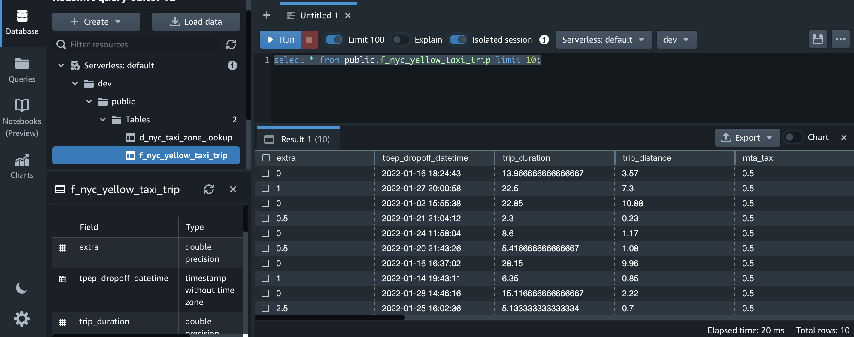
24. First, we count the number of records and select a few rows in both the target tables (f_nyc_yellow_taxi_trip and d_nyc_taxi_zone_lookup):

    SELECT 'f_nyc_yellow_taxi_trip' AS table_name, COUNT(1) FROM "public"."f_nyc_yellow_taxi_trip"
    UNION ALL
    SELECT 'd_nyc_taxi_zone_lookup' AS table_name, COUNT(1) FROM "public"."d_nyc_taxi_zone_lookup";

    

    The number of records in f_nyc_yellow_taxi_trip (2,463,931) and d_nyc_taxi_zone_lookup (265) match the number of records in our input dynamic frame. This validates that all records from files in Amazon S3 have been successfully loaded into Amazon Redshift.

    You can view some of the records for each table with the following commands:

    SELECT * FROM public.f_nyc_yellow_taxi_trip LIMIT 10;

    

    SELECT * FROM public.d_nyc_taxi_zone_lookup LIMIT 10;

    

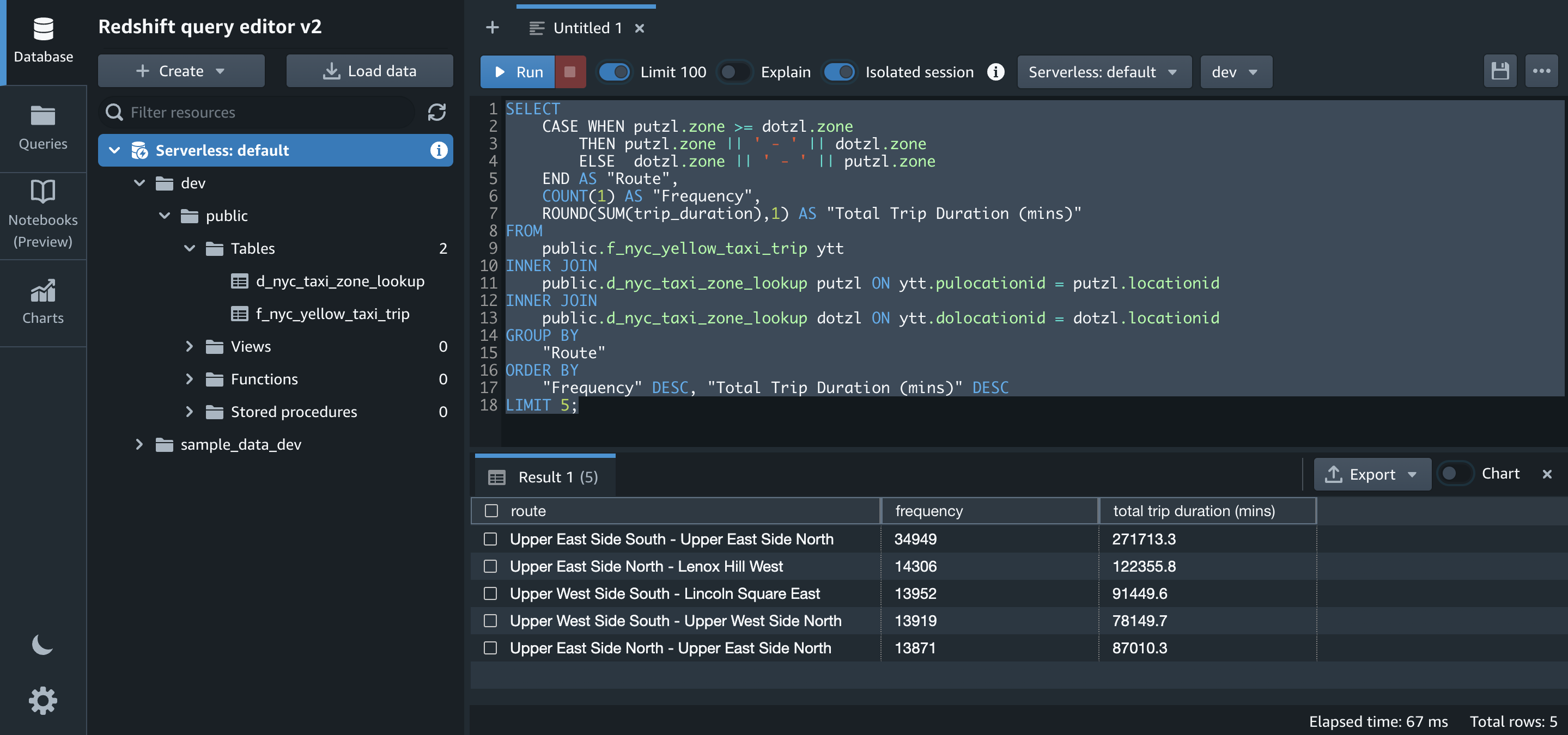
25. One of the insights that we want to generate from the datasets is to get the top five routes with their trip duration. Let’s run the SQL for that on Amazon Redshift:

    SELECT 
        CASE WHEN putzl.zone >= dotzl.zone 
            THEN putzl.zone || ' - ' || dotzl.zone 
            ELSE  dotzl.zone || ' - ' || putzl.zone 
        END AS "Route",
        COUNT(1) AS "Frequency",
        ROUND(SUM(trip_duration),1) AS "Total Trip Duration (mins)"
    FROM 
        public.f_nyc_yellow_taxi_trip ytt
    INNER JOIN 
        public.d_nyc_taxi_zone_lookup putzl ON ytt.pulocationid = putzl.locationid
    INNER JOIN 
        public.d_nyc_taxi_zone_lookup dotzl ON ytt.dolocationid = dotzl.locationid
    GROUP BY 
        "Route"
    ORDER BY 
        "Frequency" DESC, "Total Trip Duration (mins)" DESC
    LIMIT 5;

    

Transform the notebook into an AWS Glue job and schedule it

Now that we have authored the code and tested its functionality, let’s save it as a job and schedule it.

Let’s first enable job bookmarks. Job bookmarks help AWS Glue maintain state information and prevent the reprocessing of old data. With job bookmarks, you can process new data when rerunning on a scheduled interval.

1. Add the following magic command after the first cell that contains other magic commands initialized during authoring the code:

   %%configure
   {
       "--job-bookmark-option": "job-bookmark-enable"
   }

   To initialize job bookmarks, we run the following code with the name of the job as the default argument (myFirstGlueISProject for this post). Job bookmarks store the states for a job. You should always have job.init() in the beginning of the script and the job.commit() at the end of the script. These two functions are used to initialize the bookmark service and update the state change to the service. Bookmarks won’t work without calling them.

2. Add the following piece of code after the boilerplate code:

   params = []
   if '--JOB_NAME' in sys.argv:
       params.append('JOB_NAME')
   args = getResolvedOptions(sys.argv, params)
   if 'JOB_NAME' in args:
       jobname = args['JOB_NAME']
   else:
       jobname = "myFirstGlueISProject"
   job.init(jobname, args)

3. Then comment out all the lines of code that were authored to verify the desired outcome and aren’t necessary for the job to deliver its purpose:

   #nyc_taxi_trip_input_df = nyc_taxi_trip_input_dyf.toDF()
   #nyc_taxi_trip_input_df.count()
   #nyc_taxi_trip_input_df.printSchema()
   #nyc_taxi_trip_input_df.show(5)
   
   #nyc_taxi_zone_lookup_df = nyc_taxi_zone_lookup_dyf.toDF()
   #nyc_taxi_zone_lookup_df.count()
   #nyc_taxi_zone_lookup_df.printSchema()
   #nyc_taxi_zone_lookup_df.show(5)
   
   #nyc_taxi_trip_apply_mapping_dyf.toDF().printSchema()
   #nyc_taxi_zone_lookup_apply_mapping_dyf.toDF().printSchema()
   
   #nyc_taxi_trip_final_df = nyc_taxi_trip_final_dyf.toDF()
   #nyc_taxi_trip_final_df.count()
   #nyc_taxi_trip_final_df.printSchema()
   #nyc_taxi_trip_final_df.show(5)

4. Save the notebook.
   
   You can check the corresponding script on the Script tab.Note that job.commit() is automatically added at the end of the script.Let’s run the notebook as a job.
5. First, truncate f_nyc_yellow_taxi_trip and d_nyc_taxi_zone_lookup tables in Amazon Redshift using the query editor v2 so that we don’t have duplicates in both the tables:

   truncate "public"."f_nyc_yellow_taxi_trip";
   truncate "public"."d_nyc_taxi_zone_lookup";

6. Choose Run to run the job.
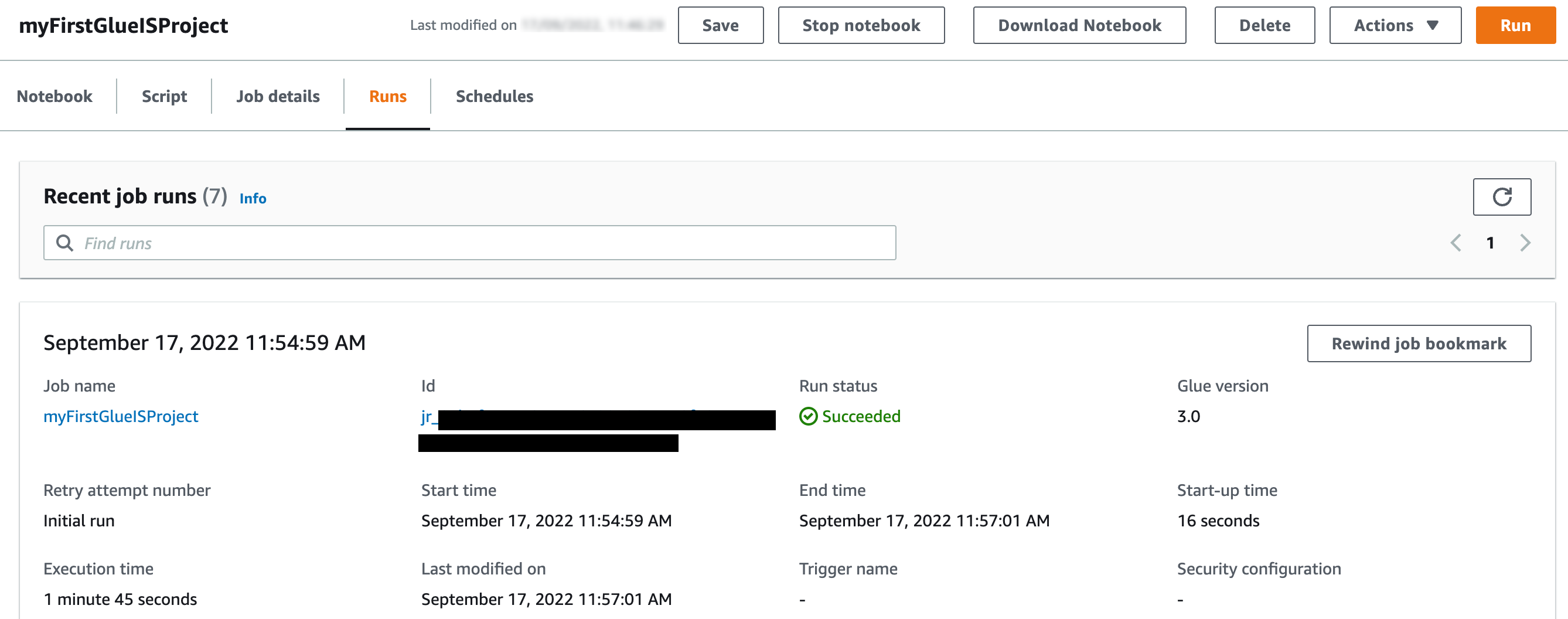
   You can check its status on the Runs tab.The job completed in less than 5 minutes with G1.x 3 DPUs.
7. Let’s check the count of records in f_nyc_yellow_taxi_trip and d_nyc_taxi_zone_lookup tables in Amazon Redshift:

   SELECT 'f_nyc_yellow_taxi_trip' AS table_name, COUNT(1) FROM "public"."f_nyc_yellow_taxi_trip"
   UNION ALL
   SELECT 'd_nyc_taxi_zone_lookup' AS table_name, COUNT(1) FROM "public"."d_nyc_taxi_zone_lookup";

   

   With job bookmarks enabled, even if you run the job again with no new files in corresponding folders in the S3 bucket, it doesn’t process the same files again. The following screenshot shows a subsequent job run in my environment, which completed in less than 2 minutes because there were no new files to process.

   

   Now let’s schedule the job.

8. On the Schedules tab, choose Create schedule.
   
9. For Name¸ enter a name (for example, myFirstGlueISProject-testSchedule).
10. For Frequency, choose Custom.
11. Enter a cron expression so the job runs every Monday at 6:00 AM.
12. Add an optional description.
13. Choose Create schedule.
    

The schedule has been saved and activated. You can edit, pause, resume, or delete the schedule from the Actions menu.

Clean up

To avoid incurring future charges, delete the AWS resources you created.

• Delete the AWS Glue job (myFirstGlueISProject for this post).
• Delete the Amazon S3 objects and bucket (my-first-aws-glue-is-project-<random number> for this post).
• Delete the AWS IAM policies and roles (AWSGlueInteractiveSessionPassRolePolicy, AmazonS3Access-MyFirstGlueISProject and AWSGlueServiceRole-GlueIS).
• Delete the Amazon Redshift tables (f_nyc_yellow_taxi_trip and d_nyc_taxi_zone_lookup).
• Delete the AWS Glue JDBC Connection (redshiftServerless).
• Also delete the self-referencing Redshift Serverless security group, and Amazon S3 endpoint (if you created it while following the steps for this post).

Conclusion

In this post, we demonstrated how to do the following:

• Set up an AWS Glue Jupyter notebook with interactive sessions
• Use the notebook’s magics, including the AWS Glue connection onboarding and bookmarks
• Read the data from Amazon S3, and transform and load it into Amazon Redshift Serverless
• Configure magics to enable job bookmarks, save the notebook as an AWS Glue job, and schedule it using a cron expression

The goal of this post is to give you step-by-step fundamentals to get you going with AWS Glue Studio Jupyter notebooks and interactive sessions. You can set up an AWS Glue Jupyter notebook in minutes, start an interactive session in seconds, and greatly improve the development experience with AWS Glue jobs. Interactive sessions have a 1-minute billing minimum with cost control features that reduce the cost of developing data preparation applications. You can build and test applications from the environment of your choice, even on your local environment, using the interactive sessions backend.

Interactive sessions provide a faster, cheaper, and more flexible way to build and run data preparation and analytics applications. To learn more about interactive sessions, refer to Job development (interactive sessions), and start exploring a whole new development experience with AWS Glue. Additionally, check out the following posts to walk through more examples of using interactive sessions with different options:

• Introducing AWS Glue interactive sessions for Jupyter
• Author AWS Glue jobs with PyCharm using AWS Glue interactive sessions
• Interactively develop your AWS Glue streaming ETL jobs using AWS Glue Studio notebooks
• Prepare data at scale in Amazon SageMaker Studio using serverless AWS Glue interactive sessions

About the Authors

Vikas Omer is a principal analytics specialist solutions architect at Amazon Web Services. Vikas has a strong background in analytics, customer experience management (CEM), and data monetization, with over 13 years of experience in the industry globally. With six AWS Certifications, including Analytics Specialty, he is a trusted analytics advocate to AWS customers and partners. He loves traveling, meeting customers, and helping them become successful in what they do.

Noritaka Sekiyama is a Principal Big Data Architect on the AWS Glue team. He enjoys collaborating with different teams to deliver results like this post. In his spare time, he enjoys playing video games with his family.

Gal Heyne is a Product Manager for AWS Glue and has over 15 years of experience as a product manager, data engineer and data architect. She is passionate about developing a deep understanding of customers’ business needs and collaborating with engineers to design elegant, powerful and easy to use data products. Gal has a Master’s degree in Data Science from UC Berkeley and she enjoys traveling, playing board games and going to music concerts.