Creating Amazon Timestream interpolated views using Amazon Kinesis Data Analytics for Apache Flink

August 30, 2023: Amazon Kinesis Data Analytics has been renamed to Amazon Managed Service for Apache Flink. Read the announcement in the AWS News Blog and learn more.

Many organizations have accelerated their adoption of stream data processing technologies in an effort to more quickly derive actionable insights from their data. Frequently, it is required that data from streams be computed into metrics or aggregations and stored in near real-time for analysis. These computed values should be generated and stored as quickly as possible; however, in instances where late arriving data is in the stream, the values must be recomputed and the original records updated.

To accommodate this scenario, Amazon Timestream now supports upsert operations, meaning records are inserted into a table if they don’t already exist, or updated if they do. The default write behavior of Timestream follows the first writer wins semantics, wherein data is stored as append only and any duplicate records are rejected. However, in some applications, last writer wins semantics or the update of existing records are required.

This post is part of a series demonstrating a variety of techniques for collecting, aggregating, and streaming data into Timestream across a variety of use cases. In this post, we demonstrate how to use the new upsert capability in Timestream to deal with late arriving data. For our example use case, we ingest streaming data, perform aggregations on the data stream, write records to Timestream, and handle late arriving data by updating any existing partially computed aggregates. We will also demonstrate how to use Amazon QuickSight for dashboarding and visualizations.

Solution overview

Time series is a common data format that describes how things change over time. Some of the most common sources of time series data are industrial machines and internet of things (IoT) devices, IT infrastructure stacks (such as hardware, software, and networking components), and applications that share their results over time. Timestream makes it easy to ingest, store, and analyze time series data at any scale.

One common application of time series data is IoT data, where sensors may emit data points at a very high frequency. IoT sensors can often introduce noise into the data source, which may obfuscate trends. You may be pushing metrics at second or sub-second intervals, but want to query data at a coarser granularity to smooth out the noise. This is often accomplished by creating aggregations, averages, or interpolations over a longer period of time to smooth out and minimize the impact of noisy blips in the data. This can present a challenge, because performing interpolations and aggregations at read time can often increase the amount of computation necessary to complete a query.

To solve this problem, we show you how to build a streaming data pipeline that generates aggregations when writing source data into Timestream. This enables more performant queries, because Timestream no longer has to calculate these values at runtime. The following diagram illustrates our solution’s architecture.

The following diagram illustrates our solution’s architecture.

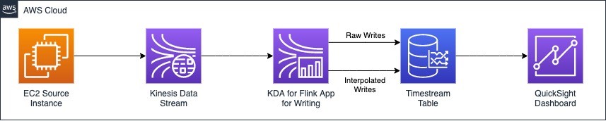
In this post, we use synthetic Amazon Elastic Compute Cloud (Amazon EC2) instance data generated by a Python script. The data is written from an EC2 instance to an Amazon Kinesis Data Streams stream. Next, a Flink application (running within Amazon Kinesis Data Analytics for Apache Flink) reads the records from the data stream and writes them to Timestream. Inside the Flink application is where the magic of the architecture really happens. We then query and analyze the Timestream data using QuickSight.

Prerequisites

This post assumes the following prerequisites:

QuickSight is set up within your account. If QuickSight is not yet set up within your account, refer to Getting Started with Data Analysis in Amazon QuickSight for a comprehensive walkthrough.
You have an Amazon EC2 key pair. For information on creating an EC2 key pair, see Amazon EC2 key pairs and Linux instances.

Setting up your resources

To get started with this architecture, complete the following steps:

Note: This solution may incur costs; please check the pricing pages related to the services we’re using.

Run the following AWS CloudFormation template in your AWS account:

For Stack name¸ enter a name for your stack.
For VPC, enter a VPC for your EC2 instance.
For Subnet, enter a subnet in which to launch your instance.

For Subnet, enter a subnet in which to launch your instance.

For KeyName, choose an EC2 key pair that may be used to connect to the instance.

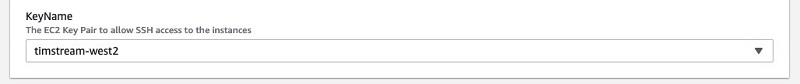
For KeyName, choose an EC2 key pair that may be used to connect to the instance.

Leave all other parameters at the default value and create the stack.

The template starts by setting up the necessary AWS Identity and Access Management (IAM) policies and roles to ensure a secure environment. It then sets up an EC2 instance and installs the necessary dependencies (Maven, Flink, and code resources) onto the instance. We also set up a Kinesis data stream and a Kinesis Data Analytics application. Later in this post, you build the Flink application and deploy it to the Kinesis Data Analytics application. The CloudFormation template also deploys the Timestream database and its corresponding Timestream table. QuickSight is not deployed via CloudFormation; we configure it manually in a later step.

The entire process of creating the infrastructure takes approximately 5 minutes. After the CloudFormation template is deployed, we have an EC2 instance, Kinesis data stream, empty Kinesis Data Analytics application, Timestream database, and Timestream table.

In the following steps, we go through setting up, compiling, and deploying the Flink application from the EC2 instance to Kinesis Data Analytics, starting the Kinesis Data Analytics application, streaming data to the Kinesis data stream, and reading the data from Timestream via interactive queries and QuickSight.

Throughout this guide, we refer to a few values contained in the Outputs section of the CloudFormation template, including how to connect to the instance, as well as the Amazon Simple Storage Service (Amazon S3) bucket used.

Building the Flink application

Let’s begin by connecting to the instance.

On the Outputs tab of the CloudFormation template, choose the link associated with ConnectToInstance.
This opens a browser-based terminal session to the instance.The EC2 instance has undergone some initial configuration. Specifically, the CloudFormation template downloads and installs Java, Maven, Flink, and clones the amazon-timestream-tools repository from GitHub. The GitHub repo is a set of tools to help you ingest data and consume data from Timestream. We use the Flink connector included in this repository as the starting point for our application.

Navigate to the correct directory, using the following command:

sudo su - ec2-user 
cd /home/ec2-user/amazon-timestream-tools/integrations/flink_connector_with_upserts

Examine the contents of the main class of the Flink job using the following command:
```
cat src/main/java/com/amazonaws/services/kinesisanalytics/StreamingJob.java
```
This code reads in the input parameters and sets up the environment. We set up the Kinesis consumer configuration, configure the Kinesis Data Streams source, and read records from the source into the input object, which contain non-aggregated records.

To produce the aggregated output, the code filters the records to only those where the measure value type is numeric. Next, timestamps and watermarks are assigned to allow for Flink’s event time processing. Event time processing allows us to operate on an event’s actual timestamp, as opposed to system time or ingestion time. For more information about event time, see Tracking Events in Kinesis Data Analytics for Apache Flink Using the DataStream API. The keyBy operation then groups records by the appropriate fields—much like the SQL GROUP BY statement. For this dataset, we aggregate by all dimensions (such as instance_name, process_name, and jdk_version) for a given measure name (such as disk_io_writes or cpu_idle). The aggregation window and the allowed lateness of data within our stream is then set before finally applying a custom averaging function.

This code generates average values for each key, as defined in the keyBy function, which is written to a Timestream table at the end of every window (with a default window duration of 5 minutes). If data arrives after the window has already passed, the allowedLateness method allows us to keep that previous window in state for the duration of the window plus the duration of allowed lateness—for example, a 5-minute window plus 2 minutes of allowed lateness. When data arrives late but within the allowed lateness, the aggregate value is recomputed to include the newly added data. The previously computed aggregate stored within Timestream must then be updated.To write data from both the non-aggregated and aggregated streams to Timestream, we use a TimestreamSink. To see how data is written and upserted within Timestream, examine the TimestreamSink class using to following command:
```
cat src/main/java/com/amazonaws/services/timestream/TimestreamSink.java
```
Towards the bottom of the file, you can find the invoke method (also provided below). Within this method, records from the data stream are buffered and written to Timestream in batch to optimize the cost of write operations. The primary thing of note is the use of the withVersion method when constructing the record to be written to Timestream. Timestream stores the record with the highest version. When you set the version to the current timestamp and include the version in the record definition, any existing version of a given record within Timestream is updated with the most recent data. For more information about inserting and upserting data within Timestream, see Write data (inserts and upserts).
```
    @Override
    public void invoke(TimestreamPoint value, Context context) throws Exception {
        List<Dimension> dimensions = new ArrayList<>();

        for(Map.Entry<String, String> entry : value.getDimensions().entrySet()) {
            Dimension dim = new Dimension().withName(entry.getKey()).withValue(entry.getValue());
            dimensions.add(dim);
        }

        //set vesion to current time
        long version = System.currentTimeMillis();

        Record measure = new Record()
                .withDimensions(dimensions)
                .withMeasureName(value.getMeasureName())
                .withMeasureValueType(value.getMeasureValueType())
                .withMeasureValue(value.getMeasureValue())
                .withTimeUnit(value.getTimeUnit())
                .withTime(String.valueOf(value.getTime()))
                //by setting the version to the current time, latest record will overwrite any existing earlier records
                .withVersion(version);

        bufferedRecords.add(measure);

        if(shouldPublish()) {
            WriteRecordsRequest writeRecordsRequest = new WriteRecordsRequest()
                    .withDatabaseName(this.db)
                    .withTableName(this.table)
                    .withRecords(bufferedRecords);

            try {
                WriteRecordsResult writeRecordsResult = this.writeClient.writeRecords(writeRecordsRequest);
                LOG.debug("writeRecords Status: " + writeRecordsResult.getSdkHttpMetadata().getHttpStatusCode());
                bufferedRecords.clear();
                emptyListTimetamp = System.currentTimeMillis();

            }   catch (RejectedRecordsException e){
                List<RejectedRecord> rejectedRecords = e.getRejectedRecords();
                LOG.warn("Rejected Records -> " + rejectedRecords.size());

                for (int i = rejectedRecords.size()-1 ; i >= 0 ; i-- ) {

                    LOG.warn("Discarding Malformed Record ->" + rejectedRecords.get(i).toString());
                    LOG.warn("Rejected Record Reason ->" + 	rejectedRecords.get(i).getReason());
                    bufferedRecords.remove(rejectedRecords.get(i).getRecordIndex());

                }
            }   catch (Exception e) {
                LOG.error("Error: " + e);
            }
        }
    }
```
Now that we have examined the code, we can proceed with compiling and packaging for deployment to our Kinesis Data Analytics application.
Enter the following commands to create a JAR file we will deploy to our Flink application:
```
mvn clean compile -Dflink.version=1.11.2
mvn package -Dflink.version=1.11.2
```

Deploying, configuring, and running the application

Now that the application is packaged, we can deploy it.

Copy it to the S3 bucket created as part of the CloudFormation template (substitute <your-bucket> with the OutputBucketName from the CloudFormation stack outputs):

aws s3 cp /home/ec2-user/amazon-timestream-tools/integrations/flink_connector_with_upserts/target/timestreamsink-1.0-SNAPSHOT.jar s3://<your-bucket>/timestreamsink/timestreamsink-1.0-SNAPSHOT.jar

We can now configure the Kinesis Data Analytics application.

On the Kinesis console, choose Analytics applications.

You should see the Kinesis Data Analytics application created via the CloudFormation template.

Choose the application and choose Configure.

We now set the code location for the Flink application.

For Amazon S3 bucket, choose the bucket created by the CloudFormation template.
For Path to Amazon S3 object, enter timestreamsink/timestreamsink-1.0-SNAPSHOT.jar.

For IAM role¸ choose the role created by the CloudFormation template.

Under Properties, expand the key-value pairs associated with FlinkApplicationProperties.

The Kinesis data stream, Timestream database, and table parameters for your Flink application have been prepopulated by the CloudFormation template.

Choose Update.

With the code location set, we can now run the Kinesis Data Analytics application.

Choose Run.
Choose Run without snapshot.

The application takes a few moments to start, but once it has started, we can see the application graph on the console.

Now that the application is running, we can start pushing data to the Kinesis data stream.

Generating and sending data

To generate synthetic data to populate the Timestream table, you utilize a script from Amazon Timestream Tools. This Git repository contains sample applications, plugins, notebooks, data connectors, and adapters to help you get started with Timestream and enable you to use Timestream with other tools and services. The Timestream Tools repository has already been cloned to the EC2 instance.

From your EC2 instance, navigate to the Timestream Tools Kinesis ingestor directory:

cd /home/ec2-user/amazon-timestream-tools/tools/kinesis_ingestor

The timestream_kinesis_data_gen.py script generates a continuous stream of EC2 instance data and sends this data as records to the Kinesis data stream. Note the percent-late and late-time parameters—these send 5% of all records 75 seconds late, leading some aggregate values to be recomputed and upserted within Timestream:

python3 timestream_kinesis_data_gen.py --percent-late 5 --late-time 75 --stream <your-kinesis-data-stream-name> --region <your-region> > writer.log &

The Flink application starts to continuously read records from the Kinesis data stream and write them to your Timestream table. Non-aggregated records are written to Timestream immediately. Aggregated records are processed and written to Timestream every 5 minutes, with aggregates recomputed and upserted when late arriving data is generated by the Python script.

Querying and visualizing your data

We can now visualize the data coming in and explore it via the Timestream console.

On the Timestream console, choose Query editor.
For Database, choose your database.

Run a quick query to verify we’re pushing both real-time and aggregated metrics:

SELECT * FROM "InterpolatedBlogDB-<xxxx>"."EC2MetricTable-<xxxx>" WHERE measure_name IN ('cpu_idle', 'avg_cpu_idle') LIMIT 100

The following screenshot shows our output.

In addition to simply querying the data, you can use QuickSight to analyze and publish data dashboards that contain your Timestream data. First, we need to ensure QuickSight has access to Timestream.

Navigate to the QuickSight console.
Choose your user name on the application bar and ensure you’re in the same Region as your Timestream database.
Choose Manage QuickSight.
Choose Security & permissions.
Ensure that Timestream is listed under QuickSight access to AWS services.
If Timestream is not listed, choose Add or remove to add Timestream.

9. If Timestream is not listed, choose Add or remove to add Timestream.

After you validate that QuickSight is configured to access Timestream, navigate to Datasets.
Choose New dataset.
Select Timestream.
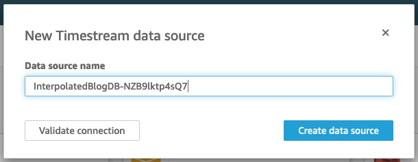
For Data source name, enter the Timestream database that was created as part of the CloudFormation template.
Choose Create data source.

Choose Create data source.

For Database, choose the database created as part of the CloudFormation template.
For Tables, select the table created as part of the CloudFormation template.
Choose Select.

Choose Select.

In the following window, choose Visualize.
When your data has loaded, choose Line chart under Visual types.
Drag the time field to the X axis
For Aggregate, choose Minute.
For Value, choose measure_value::double.
For Aggregate, select Average.
For Color, choose measure_name.

For Color, choose measure_name.

Because our Timestream data is structured as a narrow table, we need to apply filters to the dataset to select the measures of interest.

On the navigation pane, choose Filter.
Choose Create one.
Choose measure_name.
Choose the newly created filter and select avg_cpu_system and cpu_system.
Choose Apply.

The filter is now reflected in the visualization.

Conclusion

In this post, we demonstrated how to generate aggregations of streaming data, write streaming data and aggregations to Timestream, and generate visualizations of time series data using QuickSight. Through the use of Kinesis Data Streams and Kinesis Data Analytics, we deployed a data pipeline that ingests source data, and consumes this data into a Flink application that continuously reads and processes the streaming data and writes the raw and aggregated data to Timestream. We aggregated the data stream as it’s written to Timestream to reduce the amount of computation required when querying the data. With QuickSight, we rapidly developed visualizations from data stored in Timestream.

We invite you to try this solution for your own use cases and to read the following posts, which contain further information and resources:

This post is part of a series describing techniques for collecting, aggregating, and streaming data to Timestream across a variety of use cases. This post focuses on challenges associated with late arriving data, partial aggregates, and upserts into Timestream. Stay tuned for the next post in the series where we focus on Grafana integration and a Kotlin based connector for Timestream.

About the Authors

Will Taff is a Data Lab Solutions Architect at AWS based in Anchorage, Alaska. Will helps customers design and build data, analytics, and machine learning solutions to meet their business needs. As part of the AWS Data Lab, he works with customers to rapidly develop and deploy scalable prototypes through joint engineering engagements.

John Gray is a Data Lab Solutions Architect at AWS based out of Seattle. In this role, John works with customers on their Analytics, Database and Machine Learning use cases, architects a solution to solve their business problems and helps them build a scalable prototype.