Using Fleet Training to Improve Level 3 Digital Twin Virtual Sensors with Ansys on AWS

This post contrbuted by Ross Pivovar, Solution Architect, Autonomous Computing, and Adam Rasheed, Head of Autonomous Computing at AWS, and Matt Adams, Lead Product Specialist at Ansys.

In a previous post, we shared how to build and deploy a Level 3 Digital Twin virtual sensor using an Ansys model on AWS. Virtual sensors are desirable when it is difficult to physically measure a quantity, expensive to measure, or difficult to maintain the sensor. In this post, we’ll discuss challenges with Level 3 (L3) virtual sensors and describe an improved approach using a fleet-trained L3 virtual sensor.

We used Ansys Twin Builder and Twin Deployer to build the physics model and then AWS IoT TwinMaker and the TwinFlow framework to deploy on AWS. To provide context, we use our four-level Digital Twin leveling index to help customers understand their use cases and the technologies required to achieve their desired business value.

Looking at challenges with L3 virtual sensor

L3 virtual sensors are typically based on either machine-learning (ML) models or physics-based models. ML models require large training sets to cover the full domain of possible outcomes and extrapolation can be a safety concern. Comparatively, physics-based models only require small validation sets to confirm accuracy. However, these models do not reflect environmental changes like equipment degradation or deviation from the initial assumptions used to develop the physics models.

For example, Figure 1 compares the predicted value for pressure from the L3 Digital Twin virtual sensor (orange line, labeled Level 3 DT) from the prior post to the measured pressure sensor value (blue line, labeled Measured Value). The blue shaded regions around each line represent the uncertainty in the predicted and measured values. The virtual sensor is relying on the thermodynamic model of the ideal (new) compressor and initially (< 200 days) correctly predicts the discharge pressure of the fluid post-compression.

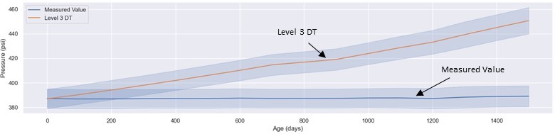
Figure 1: Graph comparing L3 DT virtual sensor prediction (without periodic calibration) versus sensor data.

As the natural gas compressor train operates in a harsh environment, the overall compressor efficiency degrades over time. The virtual sensor does not know that the compressor efficiency has decreased, and falsely predicts a higher pressure. The L3 digital twin virtual sensor (orange line) has no way to update its model parameters to improve the predictions to account for the decrease in efficiency. As a result, as shown in the graph, after 400 days, the L3 digital twin virtual sensor prediction for pressure deviated well beyond the measured sensor values (even beyond the shaded region showing the uncertainty). An operator relying on the L3 digital twin virtual sensor would mistakenly think there is a safety issue and shutdown the compressor

To alleviate this issue, operators could perform maintenance at regularly scheduled intervals, for example, every 100 days. Regular maintenance keeps the compressors running approximately at the same efficiency as new compressor trains. However, frequent maintenance is costly requiring shut-down of the facility and needs to be compared to the cost of running a compressor train in a less efficient state. Additionally, the compressor degradation depends on the environmental and operating conditions, so in some cases, doing maintenance at 100 days is too frequent, resulting in unnecessary maintenance costs. In other cases, like after a major sandstorm, maintenance is required more frequently to maintain production efficiency.

Using a fleet-trained L3 virtual sensor

An alternative is to train the model using data that includes compressor degradation, like a drop in compressor efficiency. For equipment operators running fleets of compressors, such data can be obtained from a “fleet leader” compressor that is fully instrumented. This is a common situation where the operator identifies the “fleet leader” compressor which is the oldest compressor which they intentionally fully instrument and for which they collect the most data.

In practice, simply identifying the oldest compressor is insufficient, as age is often not an ideal predictor of equipment degradation. For example, a compressor train operating in a cold, dry arctic environment degrades very differently than a compressor train operating in a hot sandy desert despite being the same age. Therefore, we need an approach that combines a physics-based understanding of the efficiency degradation with an ML model that can adjust the predictions based on the environmental and operational history of the compressor

The exact features to use for this type of adaptation depends on the physical process. In our approach, we recognize from the thermodynamics that the compressor exit pressure (P2) is a function of the temperature ratio across the compressor (T2/T1). The temperature ratio increases as the compressor degrades (for a specific pressure ratio) from physics. By incorporating this crucial piece of physics as a feature into our predictor-corrector approach (described in detail in the prior post), we’re able to improve the prediction to incorporate the compressor efficiency degradation.

We also must perform an additional step to ensure that our ML corrector model is not extrapolating beyond its training data set. Figure 2 displays the workflow for this approach for a single stage compressor. As before, the predictor model is the physics-based thermodynamic model for an ideal compressor and this time the ML corrector model is trained including the temperature ratio (T2/T1) as a feature.

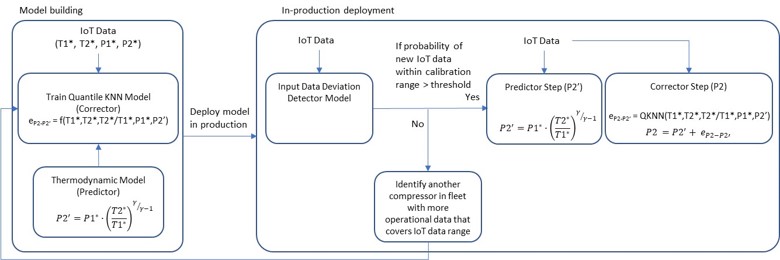
Figure 2: Workflow of a self-calibrating virtual sensor based on fleet data.

For a production model, we first perform a statistical check to calculate the probability that the model is not extrapolating beyond its training data set (Input Data Deviation Detector Model). We use a predictor-corrector model, as described in the prior post, if the model is not extrapolating. However, this time the ML corrector model includes the critical feature of temperature ratio. If we find the model is extrapolating, we trigger a model re-training by looking to the fleet for more data that covers the range of input data our compressor experiences.

As a first pass, we use data from the fully instrumented fleet leader, but with multiple fully instrumented compressors, we employ the same statistical algorithm to identify the fleet compressor with the highest probability of overlapping data. If there is no other available compressor with sufficient overlapping data, we employ a different approach of using an L4 self-calibrating virtual sensor, which we will describe in a future post.

Figure 3 shows the P2 prediction from the L3 virtual sensor model trained using the first 200 days of operation of the fully instrumented fleet leader compressor (green line). Note that this model is plotted against temperature ratio as we know it to be a better proxy for compressor performance compared to using age. For validation purposes, the orange circles show the measured P2 from our compressor during its first 200 days of operation. Normally, the orange circle data would not be available, as we would be relying on the green curve as the P2 virtual sensor prediction. As expected, we see good agreement between the measured values (orange circles) and the L3 virtual sensor.

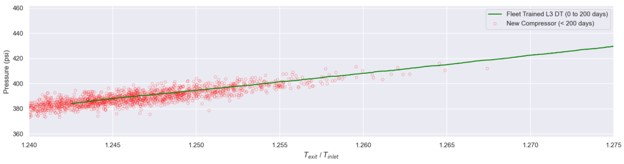
Figure 3: Graph comparing L3 DT Fleet-Trained virtual sensor prediction versus sensor data for first 200 days of operation.

However, as the compressor degrades, a higher temperature ratio doesn’t necessarily indicate higher pressure. Figure 4 shows the complete data set (0 to 1500 days of operation) from Figure 3 as our compressor efficiency degrades.

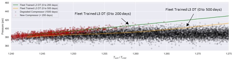
Figure 4: Graph comparing L3 DT Fleet-Trained virtual sensor predictions versus sensor data for first 200 days and 500 days of operation.

The new compressor data (<200 days of operation, red circles) is separated from the rest of the data (0 days to 1500 days of operation, black circles). In this case, we trained the ML corrector model using data from the existing fleet leader compressor that has been operating for several years (up to a temperature ratio of ~1.26). We can visually see how the improved predictor-corrector model is able to predict the compressor exit pressure up to a compressor temperature ratio of ~1.26. Beyond that, we see the prediction again deviates from the measured values indicating the ML corrector model is now extrapolating and should be retrained with a different data set. By this time, the fleet leader compressor will have likely aged and degraded further, so its dataset would presumably be suitable for training for our virtual sensor.

Identifying when the ML corrector model is extrapolating

The workflow in Figure 2 describes a crucial step of determining when the fleet-trained L3 Digital Twin model is extrapolating and needs to be retrained. For this step, we developed a function that combines Gaussian Mixture Models and Monte Carlo Integration to determine the probability that new sensor data collected by our sensors is supported by the training data set. With applying this method, we generate a training validity plot shown in Figure 5a, which shows the probability the sensor data is within the range of the training data (the first 200 days of the fleet-leader compressor). As expected, for less than 200 days, the measured sensor data exhibits a high probability of falling within the valid calibration range but then decreases over time. At approximately 200 days, the probability drops to near 0, indicating that the incoming sensor data deviated from the training set. We see this visually in Figure 5b where there is a strong overlap between the training data and the incoming sensor data for less than 100 days of operation. Conversely, Figure 5c shows poor overlap between the training data and the incoming sensor data for up to 500 days of operation.

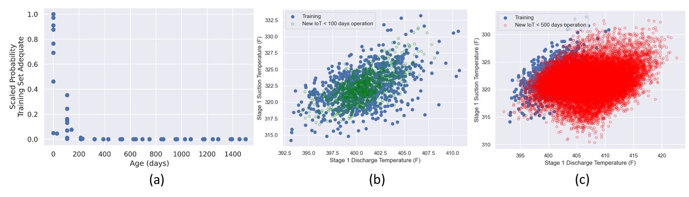
Figure 5: a) Probability new sensor data is supported by the training data using the first 200 days of data. b) Incoming sensor data overlaps the calibration data at 100 days. c) incoming sensor data does not overlap the calibration data at 500 days.

This behavior corresponds to Figure 1, where the predicted P2 values begin to deviate from the measured P2 values. Specifically, the uncertainty bands around the predicted and measured P2 no longer overlap. The Input Data Deviation model is not attempting to predict P2 or any other variable, rather it identifies when the incoming sensor data is different from the original training data.

Deploying fleet trained L3 virtual sensor on AWS

To build and deploy our L3 digital twins, we use our AWS TwinFlow framework. TwinFlow deploys and orchestrates predictive models at scale across a distributed computing architecture. It also probabilistically updates model parameters using real-world data and calculates prediction uncertainties while maintaining a fully auditable history.

In our prior post, we used TwinFlow to deploy an L3 virtual sensor when new data is added to an Amazon Simple Storage Service (Amazon S3) bucket specifying the existence of a new virtual sensor. The workflow for the prior L3 virtual sensor is shown in the “Auto-Deployment Fleet Size” and Virtual Sensors for each component” boxes in Figure 6.

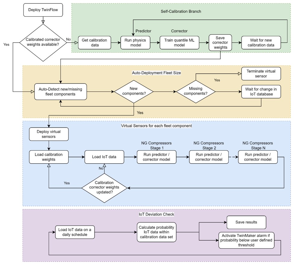
Figure 6: TwinFlow workflow enabling digital twins that auto-deploy, self-calibrate, and perform IoT sensor data deviation checks.

The Auto-Deployment box represents the workflow for auto-deployment, and the Virtual Sensors box for the initial model training. One key difference between the prior L3 virtual sensor and the present L3 fleet-trained virtual sensor is the inclusion of temperature ratio in the training feature set.

For the present implementation of the L3 fleet-trained virtual sensor, we use TwinFlow to add the additional workflows for model validity check (IoT Deviation Check box) and ML corrector model retraining (Self-Calibration box) layers as depicted in Figure 6. The model validity check runs the input data deviation detection model and displays an alarm in the AWS IoT TwinMaker dashboard when we are extrapolating beyond the training data set of the ML corrector model. If the model is found to be extrapolating, additional data is obtained from the fleet leader compressor, and the ML corrector model is retrained. If the newly trained model is still extrapolating, we adopt a more advanced approach discussed in our next post.

Figure 7 shows the AWS architecture supporting this workflow. In step 1, you download and install TwinFlow from GitHub. From here (steps 2 and 3), you can customize the virtual sensor TwinFlow pipelines and embed their digital twins in containers that are stored in Amazon Elastic Container Registry (Amazon ECR). At step 4, calibration data can be cost effectively archived in an S3 Bucket. Live sensor data is streamed into Amazon Timestream, which is a serverless database that supports real-time data. At step 5, an AWS Batch compute environment scales to meet your virtual sensors needs and optimally selects Amazon Elastic Compute Cloud (Amazon EC2) instances based on your requirements. AWS Batch supports both CPU and GPU requirements, and it elastically scales up or down based on load. In addition, all container output logs are automatically streamed to Amazon CloudWatch.

The TwinFlow graph orchestrator resides in an Amazon EC2 instance and offloads tasks to either AWS Lambda functions (which are serverless and perform short specific tasks) or directly to EC2 instances in AWS Batch. At step 6, a training task is run on Batch that will check for new calibration data in an Amazon S3 data lake and initiate ML training in AWS Batch if new data exists. A Lambda function (step 7) automatically deploys new virtual sensors or removes unused virtual sensors in AWS Batch after checking the IoT sensor database.

AWS IoT TwinMaker (step 8) shows the digital twin predictions, incoming sensor data, and 3D assets. For operational excellence, at step 9 and 10 additional diagnostic logging and archiving is performed. Since we could potentially use a large number of virtual sensors, we recommend using a Lambda function to archive logs from CloudWatch to an S3 bucket. Lastly, Amazon Neptune is used with TwinFlow to log each task execution on a graph, which also records the relationship between parent and children tasks enabling root cause analysis if an error occurs in the future.

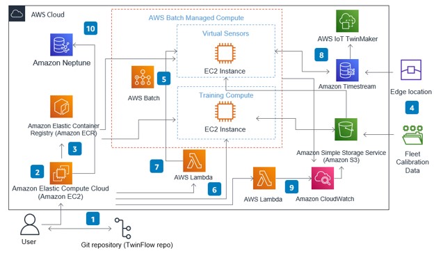
Figure 7: AWS architecture for virtual sensors.

Conclusion

In this post, we took an L3 digital twin virtual sensor workflow and added a fleet-calibration branch. We used data from the other fleet compressors to avoid having our virtual sensor extrapolate beyond its training data set. This L3 fleet-trained virtual sensor application is practical for operators running equipment fleets, like wind farms, compressor trains, oil wells, and other industrial applications. If you found this post interesting, then you should also read about a more advanced approach on deploying Level 4 digital twin self-calibrating virtual sensors.

If you want to request a proof of concept or if you have feedback on the AWS tools, please reach out to us at ask-hpc@amazon.com.

Some of the content and opinions in this blog are those of the third-party author and AWS is not responsible for the content or accuracy of this blog.