Artificial Intelligence
Remote monitoring of raw material supply chains for sustainability with Amazon SageMaker geospatial capabilities
Deforestation is a major concern in many tropical geographies where local rainforests are at severe risk of destruction. About 17% of the Amazon rainforest has been destroyed over the past 50 years, and some tropical ecosystems are approaching a tipping point beyond which recovery is unlikely.
A key driver for deforestation is raw material extraction and production, for example the production of food and timber or mining operations. Businesses consuming these resources are increasingly recognizing their share of responsibility in tackling the deforestation issue. One way they can do this is by ensuring that their raw material supply is produced and sourced sustainably. For example, if a business uses palm oil in their products, they will want to ensure that natural forests were not burned down and cleared to make way for a new palm oil plantation.
Geospatial analysis of satellite imagery taken of the locations where suppliers operate can be a powerful tool to detect problematic deforestation events. However, running such analyses is difficult, time-consuming, and resource-intensive. Amazon SageMaker geospatial capabilities provide a new and much simpler solution to this problem. The tool makes it easy to access geospatial data sources, run purpose-built processing operations, apply pre-trained ML models, and use built-in visualization tools faster and at scale.
In this post, you will learn how to use SageMaker geospatial capabilities to easily baseline and monitor the vegetation type and density of areas where suppliers operate. Supply chain and sustainability professionals can use this solution to track the temporal and spatial dynamics of unsustainable deforestation in their supply chains. Specifically, the guidance provides data-driven insights into the following questions:
- When and over what period did deforestation occur – The guidance allows you to pinpoint when a new deforestation event occurred and monitor its duration, progression, or recovery
- Which type of land cover was most affected – The guidance allows you to pinpoint which vegetation types were most affected by a land cover change event (for example, tropical forests or shrubs)
- Where specifically did deforestation occur – Pixel-by-pixel comparisons between baseline and current satellite imagery (before vs. after) allow you to identify the precise locations where deforestation has occurred
- How much forest was cleared – An estimate on the affected area (in km2) is provided by taking advantage of the fine-grained resolution of satellite data (for example, 10mx10m raster cells for Sentinel 2)
Solution overview
The solution uses SageMaker geospatial capabilities to retrieve up-to-date satellite imagery for any area of interest with just a few lines of code, and apply pre-built algorithms such as land use classifiers and band math operations. You can then visualize results using built-in mapping and raster image visualization tooling. To derive further insights from the satellite data, the guidance uses the export functionality of Amazon SageMaker to save the processed satellite imagery to Amazon Simple Storage Service (Amazon S3), where data is cataloged and shared for custom postprocessing and analysis in an Amazon SageMaker Studio notebook with a SageMaker geospatial image. Results of these custom analyses are subsequently published and made observable in Amazon QuickSight so that procurement and sustainability teams can review supplier location vegetation data in one place. The following diagram illustrates this architecture.

The notebooks and code with a deployment-ready implementation of the analyses shown in this post are available at the GitHub repository Guidance for Geospatial Insights for Sustainability on AWS.
Example use case
This post uses an area of interest (AOI) from Brazil where land clearing for cattle production, oilseed growing (soybean and palm oil), and timber harvesting is a major concern. You can also generalize this solution to any other desired AOI.
The following screenshot displays the AOI showing satellite imagery (visible band) from the European Space Agency’s Sentinel 2 satellite constellation retrieved and visualized in a SageMaker notebook. Agricultural regions are clearly visible against dark green natural rainforest. Note also the smoke originating from inside the AOI as well as a larger area to the North. Smoke is often an indicator of the use of fire in land clearing.

NDVI as a measure for vegetation density
To identify and quantify changes in forest cover over time, this solution uses the Normalized Difference Vegetation Index (NDVI). . NDVI is calculated from the visible and near-infrared light reflected by vegetation. Healthy vegetation absorbs most of the visible light that hits it, and reflects a large portion of the near-infrared light. Unhealthy or sparse vegetation reflects more visible light and less near-infrared light. The index is computed by combining the red (visible) and near-infrared (NIR) bands of a satellite image into a single index ranging from -1 to 1.
Negative values of NDVI (values approaching -1) correspond to water. Values close to zero (-0.1 to 0.1) represent barren areas of rock, sand, or snow. Lastly, low and positive values represent shrub, grassland, or farmland (approximately 0.2 to 0.4), whereas high NDVI values indicate temperate and tropical rainforests (values approaching 1). Learn more about NDVI calculations here). NDVI values can therefore be mapped easily to a corresponding vegetation class:
By tracking changes in NDVI over time using the SageMaker built-in NDVI model, we can infer key information on whether suppliers operating in the AOI are doing so responsibly or whether they’re engaging in unsustainable forest clearing activity.
Retrieve, process, and visualize NDVI data using SageMaker geospatial capabilities
One primary function of the SageMaker Geospatial API is the Earth Observation Job (EOJ), which allows you to acquire and transform raster data collected from the Earth’s surface. An EOJ retrieves satellite imagery from a specified data source (i.e., a satellite constellation) for a specified area of interest and time period, and applies one or several models to the retrieved images.
EOJs can be created via a geospatial notebook. For this post, we use an example notebook.
To configure an EOJ, set the following parameters:
- InputConfig – The input configuration defines data sources and filtering criteria to be applied during data acquisition:
- RasterDataCollectionArn – Defines which satellite to collect data from.
- AreaOfInterest – The geographical AOI; defines Polygon for which images are to be collected (in
GeoJSONformat). - TimeRangeFilter – The time range of interest:
{StartTime: <string>, EndTime: <string> }. - PropertyFilters – Additional property filters, such as maximum acceptable cloud cover.
- JobConfig – The model configuration defines the processing job to be applied to the retrieved satellite image data. An NDVI model is available as part of the pre-built
BandMathoperation.
Set InputConfig
SageMaker geospatial capabilities support satellite imagery from two different sources that can be referenced via their Amazon Resource Names (ARNs):
- Landsat Collection 2 Level-2 Science Products, which measures the Earth’s surface reflectance (SR) and surface temperature (ST) at a spatial resolution of 30m
- Sentinel 2 L2A COGs, which provides large-swath continuous spectral measurements across 13 individual bands (blue, green, near-infrared, and so on) with resolution down to 10m.
You can retrieve these ARNs directly via the API by calling list_raster_data_collections().
This solution uses Sentinel 2 data. The Sentinel-2 mission is based on a constellation of two satellites. As a constellation, the same spot over the equator is revisited every 5 days, allowing for frequent and high-resolution observations. To specify Sentinel 2 as data source for the EOJ, simply reference the ARN:
Next, the AreaOfInterest (AOI) for the EOJ needs to be defined. To do so, you need to provide a GeoJSON of the bounding box that defines the area where a supplier operates. The following code snippet extracts the bounding box coordinates and defines the EOJ request input:
The time range is defined using the following request syntax:
Depending on the raster data collection selected, different additional property filters are supported. You can review the available options by calling get_raster_data_collection(Arn=data_collection_arn)["SupportedFilters"]. In the following example, a tight limit of 5% cloud cover is imposed to ensure a relatively unobstructed view on the AOI:
Review query results
Before you start the EOJ, make sure that the query parameters actually result in satellite images being returned as a response. In this example, the ApproximateResultCount is 3, which is sufficient. You may need to use a less restrictive PropertyFilter if no results are returned.
You can review thumbnails of the raw input images by indexing the query_results object. For example, the raw image thumbnail URL of the last item returned by the query can be accessed as follows: query_results['Items'][-1]["Assets"]["thumbnail"]["Href"] .
Set JobConfig
Now that we have set all required parameters needed to acquire the raw Sentinel 2 satellite data, the next step is to infer vegetation density measured in terms of NDVI. This would typically involve identifying the satellite tiles that intersect the AOI and downloading the satellite imagery for the time frame in scope from a data provider. You would then have to go through the process of overlaying, merging, and clipping the acquired files, computing the NDVI per each raster cell of the combined image by performing mathematical operations on the respective bands (such as red and near-infrared), and finally saving the results to a new single-band raster image. SageMaker geospatial capabilities provide an end-to-end implementation of this workflow, including a built-in NDVI model that can be run with a simple API call. All you need to do is specify the job configuration and set it to the predefined NDVI model:
Having defined all required inputs for SageMaker to acquire and transform the geospatial data of interest, you can now start the EOJ with a simple API call:
After the EOJ is complete, you can start exploring the results. SageMaker geospatial capabilities provide built-in visualization tooling powered by Foursquare Studio, which natively works from within a SageMaker notebook via the SageMaker geospatial Map SDK. The following code snippet initializes and renders a map and then adds several layers to it:
Once rendered, you can interact with the map by hiding or showing layers, zooming in and out, or modifying color schemes, among other options. The following screenshot shows the AOI bounding box layer superimposed on the output layer (the NDVI-transformed Sentinel 2 raster file). Bright yellow patches represent rainforest that is intact (NDVI=1), darker patches represent fields (0.5>NDVI>0), and dark-blue patches represent water (NDVI=-1).

By comparing current period values vs. a defined baseline period, changes and anomalies in NDVI can be identified and tracked over time.
Custom postprocessing and QuickSight visualization for additional insights
SageMaker geospatial capabilities come with a powerful pre-built analysis and mapping toolkit that delivers the functionality needed for many geospatial analysis tasks. In some cases, you may require additional flexibility and want to run customized post-analyses on the EOJ results. SageMaker geospatial capabilities facilitate this flexibility via an export function. Exporting EOJ outputs is again a simple API call:
Then you can download the output raster files for further local processing in a SageMaker geospatial notebook using common Python libraries for geospatial analysis such as GDAL, Fiona, GeoPandas, Shapely, and Rasterio, as well as SageMaker-specific libraries. With the analyses running in SageMaker, all AWS analytics tooling that natively integrate with SageMaker are also at your disposal. For example, the solution linked in the Guidance for Geospatial Insights for Sustainability on AWS GitHub repo uses Amazon S3 and Amazon Athena for querying the postprocessing results and making them observable in a QuickSight dashboard. All processing routines along with deployment code and instructions for the QuickSight dashboard are detailed in the GitHub repository.
The dashboard offers three core visualization components:
- A time series plot of NDVI values normalized against a baseline period, which enables you to track the temporal dynamics in vegetation density
- Full discrete distribution of NDVI values in the baseline period and the current period, providing transparency on which vegetation types have seen the largest change
- NDVI-transformed satellite imagery for the baseline period, current period, and pixel-by-pixel differences between both periods, which allows you to identify the affected regions inside the AOI
As shown in the following example, over the period of 5 years (2017-Q3 to 2022-Q3), the average NDVI of AOI decreased by 7.6% against the baseline period (Q3 2017), affecting a total area of 250.21 km2. This reduction was primarily driven by changes in high-NDVI areas (forest, rainforest), which can be seen when comparing the NDVI distributions of the current vs. the baseline period.

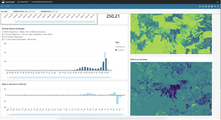
The pixel-by-pixel spatial comparison against the baseline highlights that the deforestation event occured in an area right at the center of the AOI where previously untouched natural forest has been converted into farmland. Supply chain professionals can take these data points as basis for further investigation and a potential review of relationships with the supplier in question.
Conclusion
SageMaker geospatial capabilities can form an integral part in tracking corporate climate action plans by making remote geospatial monitoring easy and accessible. This blog post focused on just one specific use case – monitoring raw material supply chain origins. Other use cases are easily conceivable. For example, you could use a similar architecture to track forest restoration efforts for emission offsetting, monitor plant health in reforestation or farming applications, or detect the impact of droughts on water bodies, among many other applications.
About the Authors
 Karsten Schroer is a Solutions Architect at AWS. He supports customers in leveraging data and technology to drive sustainability of their IT infrastructure and build cloud-native data-driven solutions that enable sustainable operations in their respective verticals. Karsten joined AWS following his PhD studies in applied machine learning & operations management. He is truly passionate about technology-enabled solutions to societal challenges and loves to dive deep into the methods and application architectures that underlie these solutions.
 Tamara Herbert is an Application Developer with AWS Professional Services in the UK. She specializes in building modern & scalable applications for a wide variety of customers, currently focusing on those within the public sector. She is actively involved in building solutions and driving conversations that enable organizations to meet their sustainability goals both in and through the cloud.
 Margaret O’Toole joined AWS in 2017 and has spent her time helping customers in various technical roles. Today, Margaret is the WW Tech Leader for Sustainability and leads a community of customer facing sustainability technical specialists. Together, the group helps customers optimize IT for sustainability and leverage AWS technology to solve some of the most difficult challenges in sustainability around the world. Margaret studied biology and computer science at the University of Virginia and Leading Sustainable Corporations at Oxford’s Saïd Business School.