Using Fewer Resources to Run Deep Learning Inference on Intel FPGA Edge Devices

By Yoshitaka Haribara, Startup ML Solutions Architect at AWS
By Joseph Glover, Partner Solutions Architect at AWS

Inference is an important stage of machine learning (ML) pipelines that deliver insights to end users from trained neural network models. These models are deployed to perform predictive tasks like image classification, object detection, and semantic segmentation.

However, constraints such as limited power consumption and heat dissipation, plus requirements for high throughput with low latency, can make implementing inference at scale on edge devices such as Internet of Things (IoT) controllers and gateways challenging.

To overcome these challenges, both hardware and software optimization are necessary. From the hardware perspective, a field-programmable gate array (FPGA) can be a good candidate. With FPGA, you can benefit from hardware acceleration of configurable logic blocks, which result in high performance per watt, low-latency, and flexibility.

Intel, an AWS Partner Network (APN) Advanced Technology Partner with the AWS IoT Competency, has a rich FPGA portfolio. Intel has proven success in application segments that require long lifecycle and reliability, including industrial and automotive.

In this post, we will show you how to train and convert a neural network model for image classification to an edge-optimized binary for Intel FPGA hardware.

Model Quantization

We mentioned how the hardware acceleration of Intel FPGA chips improves performance, latency, and flexibility. That’s only part of the story. On the software side, we can reduce the bandwidth, compute, and memory resources required for deep learning by applying model quantization.

This technique seeks to represent numbers, such as weights and activation functions, with the low-bit integers without incurring significant loss in accuracy.

Specifically, you can reduce resource usage by replacing the parameters in an inference model with half-precision (16bit), bfloat16 (16bit, but the same dynamic range as 32bit), or 8bit integers instead of the usual single-precision floating-point (32bit) values.

The limit of quantization without performance degradation is generally believed to be 8 bits, but with Blueoil, provided by LeapMind Inc., you can achieve negligible performance degradation even with a combination of 1-bit weight and 2-bit activation, well below 8 bits.

Blueoil is an open source edge deep learning framework that helps you create a neural network model for low-bit computation. Without expertise in edge deep learning, you can easily obtain an edge-optimized model in four steps: prepare the dataset, generate a configuration file, train the model, and convert the model.

In fact, the 1-bit matrix multiplication can be implemented with an XNOR gate, which dramatically improves calculation efficiency with much less memory and fewer multipliers. Intel FPGA is a suitable architecture for 1-bit because combinational logic can process gate-level signals without any overhead, and it’s configurable for its data path.

In particular, using Cyclone V SoC FPGA, you can combine an image signal processing pipeline with machine vision algorithms executing the ARM Cortex-A9 hard processor system to build a complete machine vision system on a chip with low power consumption. Such a system would be a cost-effective option for large production deployments.

It’s worth noting that general purpose computing on graphics processing units (GP-GPU) would be less efficient in this case because GPUs are typically designed to process larger and higher-precision signals such as FP32. These require larger circuit size, resulting in higher power use and cost.

Solution Overview

Our use case is an attempt to mimic an industrial computer vision application consisting of an edge gateway (a camera), and an analytics backend.

Figure 1 − Edge deep learning pipeline onto Intel FPGA.

On the left side is our target device for inference at the edge, a Terasic DE10-Nano Kit. Based on an Intel SoC FPGA, this development board provides a reconfigurable hardware design platform for makers, IoT developers, and educators. It has been qualified under AWS IoT Greengrass for the AWS Device Qualification Program (DQP), and is listed in the AWS Partner Device Catalog.

The right side of the architecture represents the AWS Cloud, where the model is trained and converted to be optimized for our target edge device.

How We Trained and Converted the Model

These are the steps we took to train and convert the model.

Prerequisites

• An AWS account.
• Terasic DE10-Nano Kit (about $140 on Amazon.com) if you actually want to try inference at the edge.
• Ethernet cable and internet connection.
• A laptop or local development environment.

To train and convert the model, we performed these steps:

1. Launched an Amazon SageMaker Notebook instance and cloned GitHub repository bluegrass.
2. Built a Docker image, prepared the dataset, set up the configuration, and trained and converted the model in a sample notebook.
3. Checked the inference results on the cloud.
4. Tried inference at the edge with Cyclone V SoC FPGA on a DE10-Nano device.

Step 1: Launch an Amazon SageMaker Notebook Instance

We prepared the quantized model using Amazon SageMaker Notebook as our development environment. Amazon SageMaker is a fully managed service that gives developers and data scientists the ability to build, train, and deploy machine learning models quickly.

To start, we logged in to the AWS Management Console and jumped to the Amazon SageMaker page.

We chose Notebook Instances from the left pane, and selected Create notebook instance.

In the next page, we entered bluegrass-notebook as the value for Notebook instance name. Then we selected the instance type (ml.t3.medium) and set an appropriate AWS Identity and Access Management (IAM) role.

Under the Repository field in the Git repositories – optional section, we entered the name of the GitHub repository shown in Figure 2 into the box that says Clone a public Git repository to.

Figure 2 – Git repositories in Amazon SageMaker.

We then selected the Create notebook instance button and waited.

After the notebook instance changed state to InService, we opened the JupyterLab environment and found blueoil_cifar10_example.ipynb. This notebook performs these actions:

• Builds a Docker image based on a Blueoil container for model training and conversion, then uploads it to Amazon Elastic Container Registry (Amazon ECR).
• Prepares data by downloading, extracting, and uploading the pre-processed dataset from a public Amazon Simple Storage Service (Amazon S3) bucket to your bucket.
• Uploads your Blueoil configuration Python file to your Amazon S3 bucket.
• Trains a model with an Amazon SageMaker training job.
• Converts the trained model with Amazon SageMaker processing.
• Downloads the converted model.

Step 2: Build a Docker Image to Run Blueoil on Amazon SageMaker

The notebook we selected builds a Docker image to run Blueoil on Amazon SageMaker and pushes it to Amazon ECR. This Docker image is used when we run Amazon SageMaker training and processing jobs.

An Amazon SageMaker training job is a fully managed training environment in which we can submit our Python script to use pre-built containers such as TensorFlow, Apache MXNet, or PyTorch. We can also bring your own container (BYOC) to the training job.

Blueoil has its own Dockerfile in the Blueoil repository. To use it for BYOC on Amazon SageMaker, we had to modify it. We had to set ENV with reserved sub-directories, COPY our Python training script, and change ENTRYPOINT so Amazon SageMaker can run the image. These modifications are executed by docker_push_ecr.sh, referencing our Dockerfile.

Preparing the Dataset

We used the publicly available CIFAR-10 dataset, which is commonly used for image classification tasks. You can also use the Open Images dataset for object detection example notebooks. There are several examples in our repository.

The CIFAR-10 dataset consists of 60,000 images in 10 classes such as airplane, automobile, and bird. While the original dataset is provided in a NumPy array format for Python, Blueoil also supports the Caltech101 format.

We downloaded the CIFAR-10 in Caltech101 format, where the 10 categories are classified in the directory structure for each set of training and testing data. For details about the data format, please refer to Prepare training dataset.

Next, we uploaded the extracted dataset to Amazon S3. Here, we implicitly specified the dataset path for an S3 bucket; in effect, our SageMaker default bucket of the form sagemaker-{region}-{AWS account ID}). This bucket is later put under /opt/ml/input/data directory in the Docker container for training.

Configuring Blueoil

Blueoil configuration is usually created by running the blueoil init command after a Blueoil installation. In our example, the cifar10_sample.py configuration file was already provided.

The configuration file specifies the input image size ([32, 32]), batch size (64), optimizer setup (momentum with specific parameters such as learning rate), quantizer configuration (binary weight, 2 bit activation), and data augmentation method.

We uploaded the configuration file to the Amazon SageMaker default bucket on S3 in the same way as the dataset.

Figure 3 – Uploading Blueoil configuration file to Amazon S3.

Using the Amazon SageMaker Training and Processing Job

We launched an Amazon SageMaker training job in SageMaker Python SDK:

import sagemaker

from sagemaker.estimator import Estimator


train_instance_type = 'ml.p3.2xlarge'


estimator = Estimator(

   image_name=ecr_image,

   role=sagemaker.get_execution_role(),

   train_instance_count=1,

   ….....

      …………….

      …………….


estimator.fit({'dataset': train_data, 'config': config_data})

The Estimator construct specifies the Docker image in Amazon ECR, the instance count, and the type. The last line invokes the training. It takes about 30 minutes to finish the job with an ml.p3.2xlarge GPU instance.

We monitored the progress by watching the logs shown in the notebook, which is also sent to Amazon CloudWatch Logs. The trained model is saved to the S3 bucket.

We converted the model in an Amazon SageMaker processing job in a similar way. The converted model and an inference script were compressed as output.tar.gz, and saved to the S3 bucket.

Processing the Training Model

Let’s dive into the Amazon SageMaker training jobs and processing jobs.

For our example, we prepared the Docker container. It contains a main.py script, which calls train and convert commands from Blueoil, and runs them in Amazon SageMaker training and processing jobs, respectively.

You can take two approaches to model quantization: quantization during training and quantization after training. The former approach trains neural networks to anticipate errors due to quantization.

Blueoil adopts quantization-aware training, which usually benefits from high accuracy even after quantization. The Blueoil convert command executes the following processes as described in Convert Training Result to FPGA-Ready Format:

• Converts the TensorFlow checkpoint to protocol buffer graph.
• Optimizes the graph.
• Generates source code for an executable binary.
• Compiles for x86-64, ARM and FPGA.

Step 3: Checking the Inference Results on the Cloud

After the training and conversion was complete, we downloaded and extracted the output.tar.gz file, which contained the model artifact. We extracted it to get the cifar10_sample directory.

The artifacts are accommodated in:

cifar10_sample/saved/{MODEL_NAME}/export/save.ckpt-{Checkpoint No.}/{Image size}/output subdirectory; namely, cifar10_sample/export/save.ckpt-78125/32x32/output/

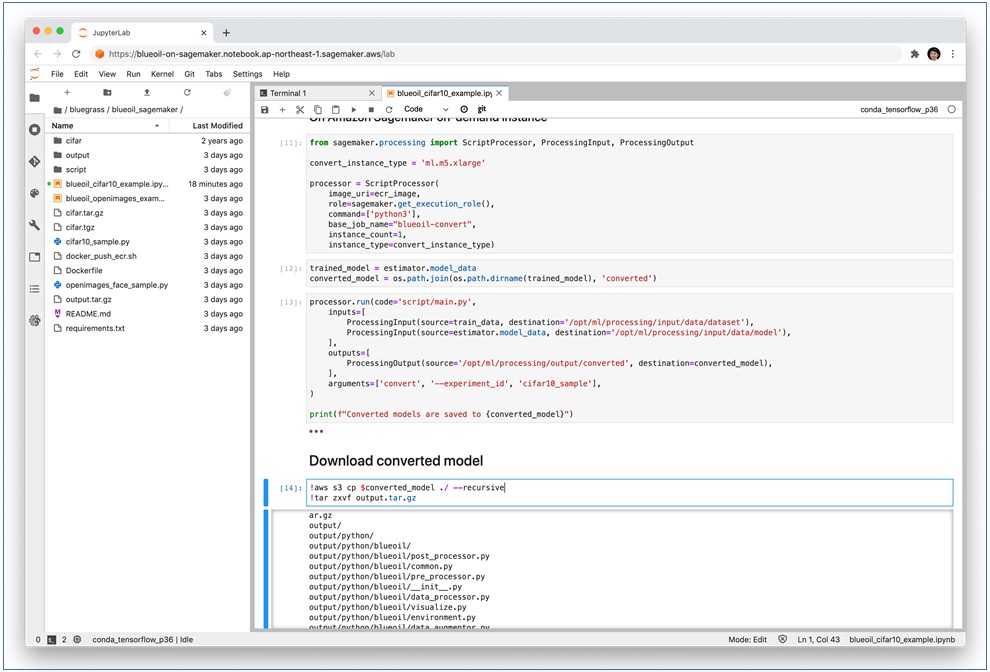
Figure 4 – Extracting the output.tar.gz file.

To check the results in the notebook instance, we opened a terminal window and ran the run.py script after running sudo pip install -r requirements.txt in output/python. Here is an example for inferring the label of this airplane image:

$ python run.py \

   -i airplane.png \

   -m ../models/lib/libdlk_x86.so \

   -c ../models/meta.yaml

It generated output/output.json.

Here are the results for an ml.m5.xlarge notebook instance:

$ cat output/output.json

{

   "benchmark": {

      "inference": 0.03394120899997688,

      "post": 0.009801765000020168,

      "pre": 0.003248117000111961,

      "total": 0.04699109100010901

   },

   "classes": [

      {

         "id": 0,

          "name": "airplane"

…..

………

………….

              "probability": "0.77472717"

The airplane class is the label predicted with the highest probability.

We used the Intel x86 architecture because Amazon SageMaker notebook instances have Intel Xeon CPUs. If you want to try this with ARM architectures, you can run a similar procedure in Amazon EC2 A1 or M6g/C6g/R6g instances with AWS Graviton/Graviton2 processors.

Here is the result for an m6g.xlarge instance, using this setup script:

$ cat output/output.json

{

   "benchmark": {

      "inference": 0.002424001693725586,

       "post": 0.009356975555419922,

      "pre": 0.0031518936157226562,

      "total": 0.014932870864868164

   },

…

   "results": [

      {

         "file_path": "airplane.png",

         "prediction": [

            {

               "class": {

                  "id": 0,

                  "name": "airplane"

               },

              "probability": "0.77472717"

It outputs the same predicted label airplane with the highest probability. You can also find libdlk_fpga.so in the model/lib directory. This is the one you’ll use on your DE10-Nano device.

Step 4: Tried Inference at the Edge

To try inference on a DE10-Nano device, you must first write the boot image to a microSD card on a host computer (your laptop or local development environment). The easiest way is to use Etcher software. Then you can set it to your DE10-Nano device and start.

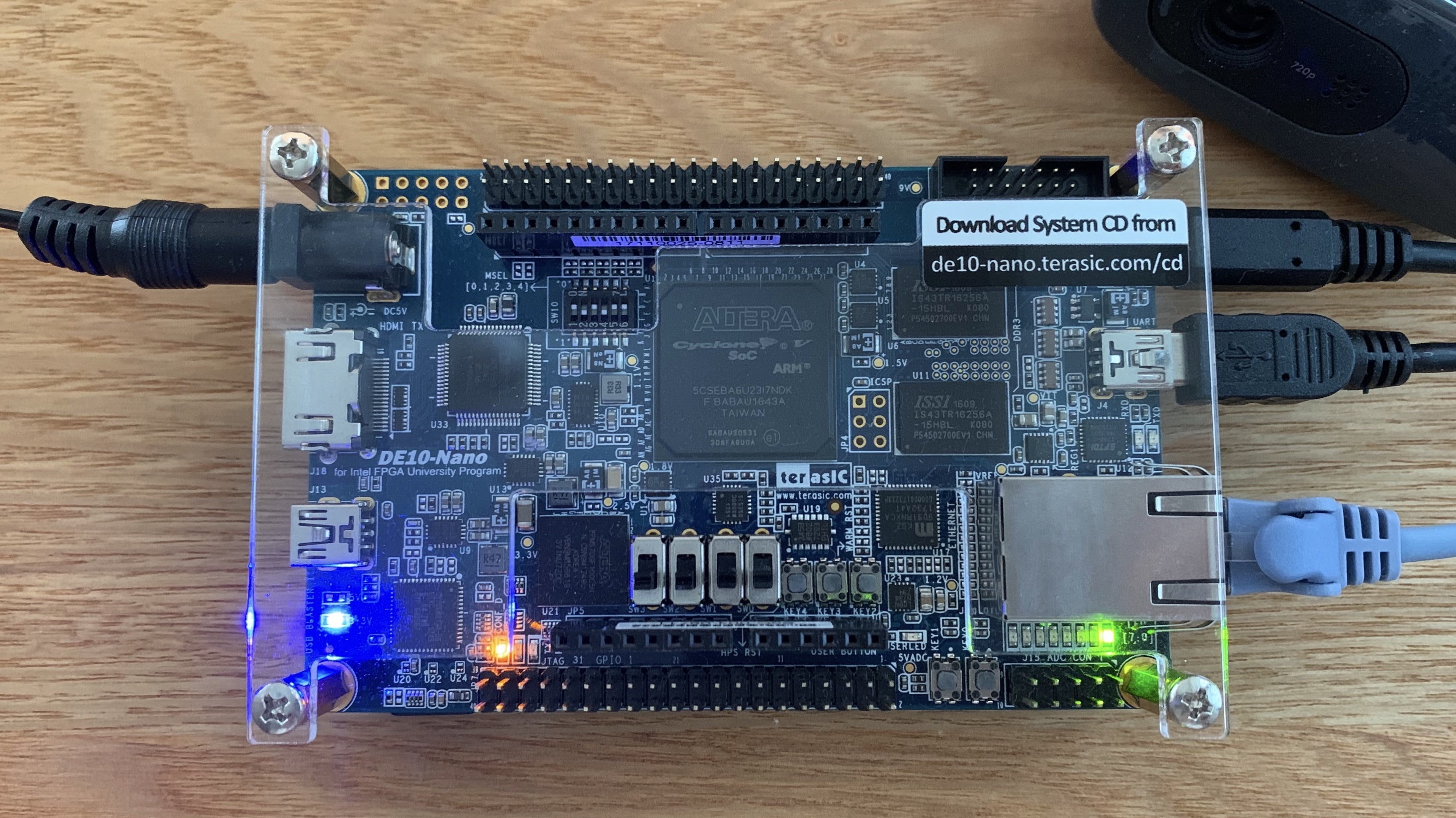
Figure 5 – Writing a boot image to a DE10-Nano device.

On the upper left of the device, a power adapter is connected. On the right side from top to bottom, there is first a USB Micro-B for a camera, and then USB Mini-B for UART connection to your host computer (optional for debugging). Finally, there is an Ethernet cable required to set up an internet connection.

You can access the device via UART, like this:

sudo cu -l  /dev/<your_fpga_board>  -s 115200

On Linux, it looks like this:

sudo cu -l  /dev/ttyUSB0  -s 115200

On MacOs, it looks like this:

sudo cu -l  /dev/tty.usbserial-A106I1IY -s 115200

The default username and password are root and de10nano, respectively.

You can also check the IP address with the ifconfig command. We recommend you first fix your IP address, which should be consistent during the setup process and with the Ansible automation engine later.

You can find your device’s MAC address with ifconfig | grep HWaddr and put the output at the end of the /etc/network/interfaces file as:

auto eth0

iface eth0 inet dhcp

hwaddress ether <MAC address of your device>

You can set up the Secure Shell Home (SSH) configuration (using ssh-keygen and ssh-copy-id).  Then, run the Ansible Playbook as in this README:

$ ansible-playbook -i <IP address of your device>, ansible/playbook.yml

This command updates the Linux kernel module, zImage, preloaders, etc., for running on Blueoil.

Finally, download output.tar.gz from Amazon S3, send it to the device, extract it, and find the cifar10_sample/export/save.ckpt-78125/32x32/output/python directory. Then, install the rest of required packages:

$ apt-get update

$ apt-get install python3-pip libjpeg-dev zlib1g-dev

$ pip3 install -r requirements.txt

Run the similar command after downloading the sample image:

$ python run.py \

-i airplane.png \

-m ../models/lib/libdlk_fpga.so \

-c ../models/meta.yaml

Here is the output:

$ cat output/output.json

{

   "benchmark": {

      "inference": 0.007309094988158904,

      "post": 0.1206085180019727,

      "pre": 0.03428893999080174,

      "total": 0.16220655298093334

   },

…

   "results": [

      {

         "file_path": "airplane.png",

         "prediction": [

            {

               "class": {

                  "id": 0,

                  "name": "airplane"

               },

               "probability": "0.9101995"

Cleaning Up

To avoid incurring future charges, delete the resources you used, such as the Amazon SageMaker notebook instance.

Conclusion

Amazon SageMaker with Blueoil trains and optimizes deep learning models for inference at the edge on Intel FPGA processors with fewer computational resources. This approach can overcome the constraints of large industrial deployments of inference at the edge by providing low latency with high throughput without sacrificing accuracy.

Our goal is to enable customers and partners to easily deploy cloud-to-edge deep learning pipelines.
.

.

Intel – APN Partner Spotlight

Intel is an AWS Competency Partner that shares a passion with AWS for delivering constant innovation. Together, Intel and AWS have developed a variety of resources and technologies for high-performance computing, big data, machine learning, and IoT.

Contact Intel | Practice Overview | AWS Marketplace

*Already worked with Intel? Rate the Partner

*To review an APN Partner, you must be an AWS customer that has worked with them directly on a project.