AWS Big Data Blog
Detect fraudulent calls using Amazon QuickSight ML insights
The financial impact of fraud in any industry is massive. According to the Financial Times article Fraud Costs Telecoms Industry $17bn a Year (paid subscription required), fraud costs the telecommunications industry $17 billion in lost revenues every year.
Fraudsters constantly look for new technologies and devise new techniques. This changes fraud patterns and makes detection difficult. Companies commonly combat this with a rules-based fraud detection system. However, once the fraudsters realize their current techniques or tools are being identified, they quickly find a way around it. Also, rules-based detection systems tend to struggle and slow down with a lot of data. This makes it difficult to detect fraud and act quickly, resulting in loss of revenue.
Overview
There are several AWS services that implement anomaly detection and could be used to combat fraud, but lets focus on the following three:
When trying to detect fraud, there are two high-level challenges:
- Scale – The amount of data to be analyzed. For example, each call generates a call detail record (CDR) event. These CDRs include many pieces of information such as originating and terminating phone numbers, and duration of call. Multiply these CDR events times the number of telephone calls placed each day and you can get an idea of the scale that operators must manage.
- Machine learning knowledge and skill – The right set of skills to help solve business problems with machine learning. Developing these skills or hiring qualified data scientists with adequate domain knowledge is not simple.
Introducing Amazon QuickSight ML Insights
Amazon QuickSight is a fast, cloud-powered BI service that makes it easy for everyone in an organization to get business insights from their data through rich, interactive dashboards. With pay-per-session pricing and a dashboard that can be embedded into your applications, BI is now even more cost-effective and accessible to everyone.
However, as the volume of data that customers generate grows daily, it’s becoming more challenging to harness their data for business insights. This is where machine learning comes in. Amazon is a pioneer in using machine learning to automate and scale various aspects of business analytics in the supply chain, marketing, retail, and finance.
ML Insights integrates proven Amazon technologies into Amazon QuickSight to provide customers with ML-powered insights beyond visualizations.
- ML-powered anomaly detection to help customers uncover hidden insights by continuously analyzing across billions of data points.
- ML-powered forecasting and what-if analysis to predict key business metrics with point-and-click simplicity.
- Auto-narratives to help customers tell the story of their dashboard in a plain-language narrative.
In this post, I demonstrate how a Telecom provider with little to no ML expertise can use Amazon QuickSight ML capabilities to detect fraudulent calls.
Prerequisites
To implement this solution, you need the following resources:
- Amazon S3 to stage a ‘ribbon’ call detail record sample in a CSV format.
- AWS Glue running an ETL job in PySpark.
- AWS Glue crawlers to discover the schema of the tables and update the AWS Glue Data Catalog.
- Amazon Athena to query the Amazon QuickSight dataset.
- Amazon QuickSight to build visualizations and perform anomaly detection using ML Insights.
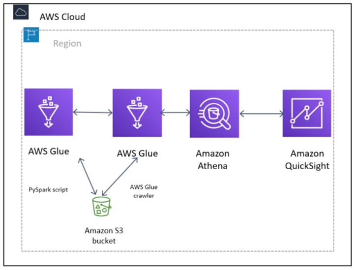
Diagram of fraudulent call-detecting architecture, using a PySpark script to prepare the data and transform it into Parquet and an AWS Glue crawler to build the AWS Glue Data Catalog.
The dataset
For this post, I use a synthetic dataset, thanks to Ribbon Communications. The data was generated by call test generators, and is not customer or sensitive data.
Inspecting the data
The example below is a typical CDR. The STOP CDR shown below is generated after a call has been terminated.
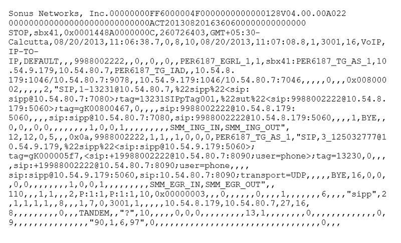
As you can see, there are a lot of values here. Most of them are not relevant for fraud identification or prevention.
Revenue shared fraud
Revenue shared fraud is one of the most common fraud schemes threatening the telecom industry today. It involves using fraudulent or stolen numbers to repeatedly call a premium rate B-number, who then shares the cash generated with the fraudster.
Say that you’d like to detect national and international revenue share fraud using Amazon QuickSight ML. Consider the typical traits of a revenue share fraud phone call. The pattern for revenue share fraud is multiple A-numbers calling the same B-number or a range of B-numbers with the same prefix. The call duration is usually higher than average and could be up to two hours, which is the maximum length of time international switches allow. Generally, the calls originate from one cell or a group of cells.
One SIM may make short test calls to a variety of B-numbers as a precursor to the fraud itself, which most often happens when the risk of detection is lowest, for example, Friday night, weekends, or holidays. Conference calling may be used to make several concurrent calls from one A-number.
Often, SIMs used for this type of fraud are sold or activated in bulk from the same distributor or group of distributors. SIMs could be topped up using fraudulent online or IVR payments, such as using stolen credit card numbers. Both PAYG credit and bundles may be used.Based on the above use case, the following pieces of information are most relevant to detecting fraud.
- Call duration
- Calling number (A number)
- Called number (B number)
- Start time of the call
- Accounting ID
You can use this reference to help identify those fields in a CDR.
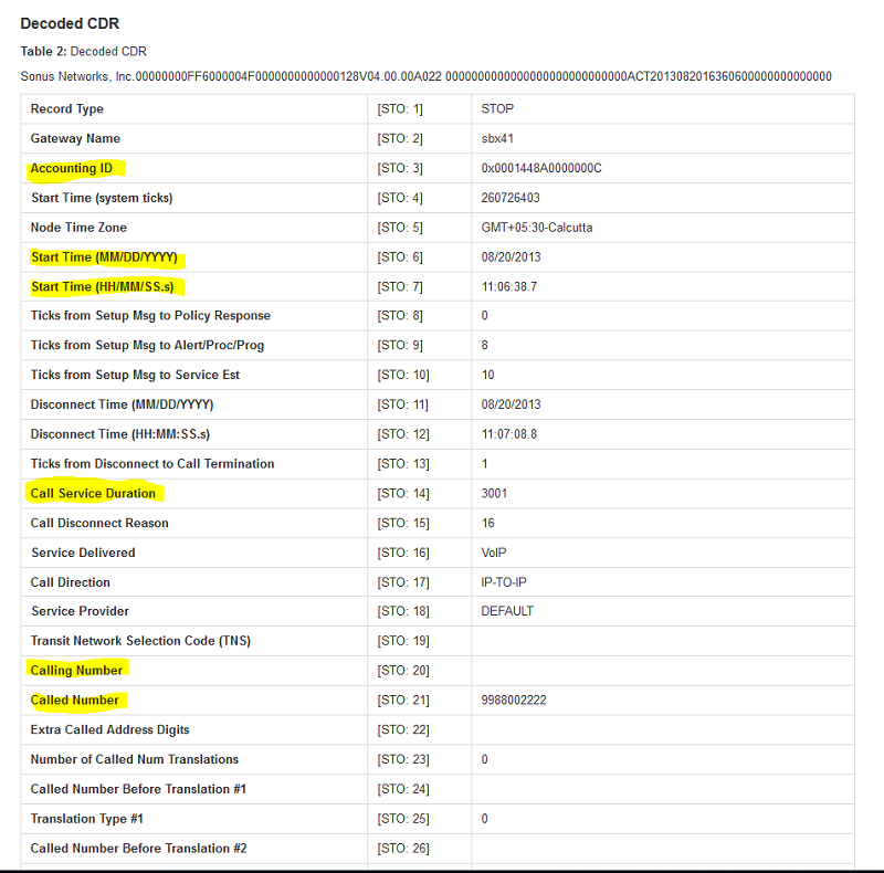
Figure 2: Decoded CDR data, highlighting the relevant fields.
I identified the columns that I need out of 235 columns in the CDR.
Inspecting the raw sample data, I quickly see that it’s missing a header.
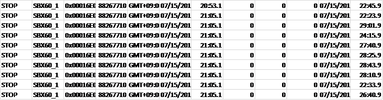
To make life easier, I converted the raw CSV data, added the column names, and converted to Parquet.
Discovering the data
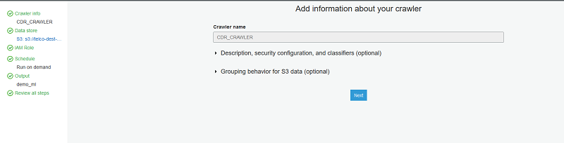
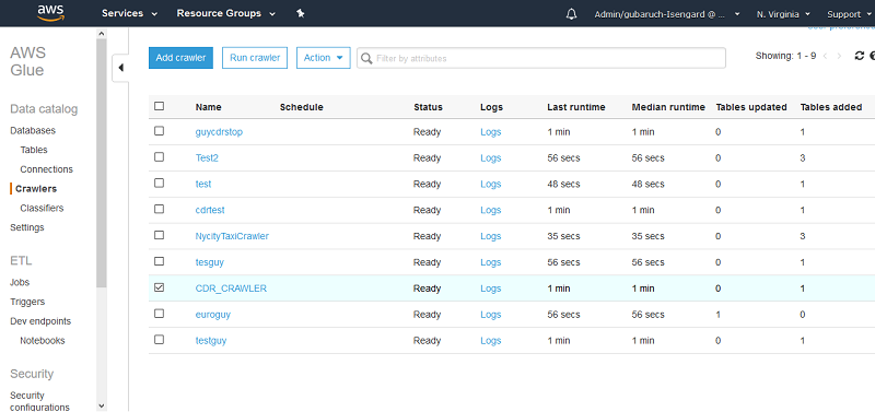
In the AWS Glue console, set up a crawler and name it CDR_CRAWLER.
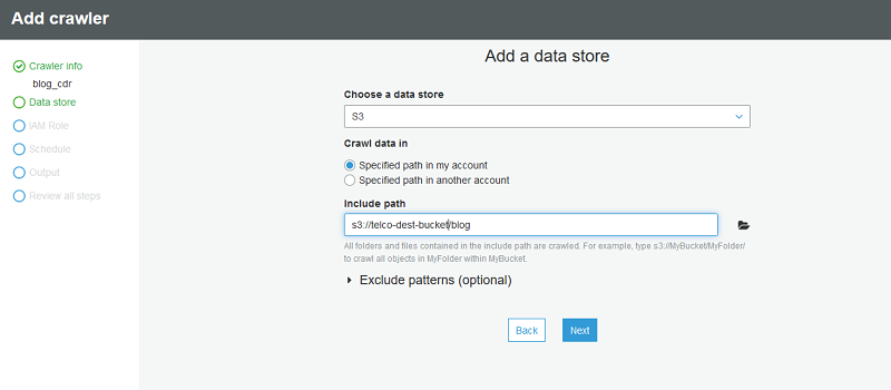
Point the crawler to s3://telco-dest-bucket/blog where the Parquet CDR data resides.
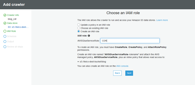
Next, create a new IAM role to be used by the AWS Glue crawler.
You need to grant your IAM role permissions that AWS Glue can assume when calling other services on your behalf. This includes access to Amazon S3 for any sources, targets, scripts, and temporary directories that you use with AWS Glue. Permission is needed by crawlers, jobs, and development endpoints.
Only use the “Managed Policies” as a starting point and modify them as per their business needs.
For Frequency, leave the default definition of Run on Demand.
Next, choose Add database and define the name of the database. This database contains the table discovered by the AWS Glue crawler.
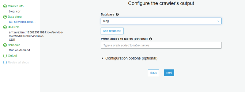
Choose next and review the crawler settings. When you’re satisfied, choose Finish.
Next, choose Crawlers, select the crawler that you just created (CDR_CRAWLER), and choose Run crawler.
The AWS Glue crawler starts crawling the database. This can take one minute or more to complete.
When it’s complete, under Data catalog, choose Databases. You should be able to see the new database created by the AWS Glue crawler. In this case, the name of the database is blog.
To view the tables created under this database, select the relevant database and choose Tables. The crawler’s table also points to the location of the Parquet format CDRs.
To see the table’s schema, select the table created by the crawler.
Data preparation
You have defined the relevant dimensions to use in the ML model to detect fraud. If you would like to practice with the data preparation part rather than using the existing processed parquet files, you can use a PySpark script that I built earlier using an Amazon SageMaker notebook and an AWS Glue endpoint. The script covers the following tasks:
- Reduce the dataset and focus only on the relevant columns.
- Create a timestamp column, which you need for creating an analysis using Amazon QuickSight.
- Transform files from CSV to Parquet for improved performance.
You can run the PySpark script on the raw CSV format of the CDRs that you are using. Here is the location of the raw CSV format:
s3://telco-source-bucket/machine-learning-for-all/v1.0.0/data/cdr-stop/cdr_stop.csv
Here is the PySpark script that I created.
The dataset has been cataloged in AWS Glue Data Catalog and is queryable using Athena.
Amazon QuickSight and anomaly detection
Next, build out anomaly detection using Amazon QuickSight. To get started, follow these steps.
- In the Amazon QuickSight console, choose new analysis.
- click on create new data set
- select Athena
- enter a data source name
- click on create data source
- select from the drop down list the relevant database and table that were created by the AWS Glue crawlers and click on select
- select directly query your data and click visualize
Visualizing the data using Amazon QuickSight
- Under visual types, choose Line chart.
- Drag call_service_duration to the Value field well.
- Drag timestamp_new to the X axis field well.
Amazon QuickSight generates a dashboard, as in the following screenshot.
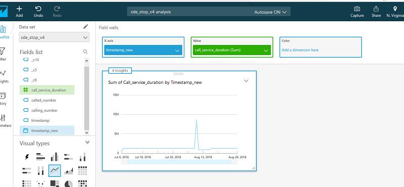
The x-axis is the timestamp. By default, it’s based on the aggregates of one day. This can be changed by choosing a different value.

Because I currently define the timestamp to look on one-day aggregations, the call duration is a sum of all call durations from all call records within a day. I can begin the search by looking for days where the total call duration is high.
Anomaly detection
Now look at how to start using the ML insights anomaly detection feature.
- On the top of the Insights panel, choose Add anomaly to sheet. This creates an insights visual for anomaly detection.
- On the top of the screen, choose Field Wells and add at least one field to the Categories, as in the following example. I added the calling/called number, as those become relevant for fraud use cases; for example, one A-number calling multiple B-numbers or multiple A-numbers calling B-numbers.

The categories represent the dimensional values by which Amazon QuickSight splits the metric. For example, you can analyze anomalies on sales across all product categories and product SKUs—assuming there are 10 product categories, each with 10 product SKUs. Amazon QuickSight splits the metric by the 100 unique combinations and runs anomaly detection on each of the split metric. - To configure the anomaly detection job, choose Get Started.
- On the anomaly detection configuration screen, set up the following options:
- Analyze all combinations of these categories—By default, if you have selected three categories, Amazon QuickSight runs anomaly detection on the following combinations hierarchically: A, AB, ABC. If you select this option, QuickSight analyzes all combinations: A, AB, ABC, BC, AC. If your data is not hierarchical, check this option.
- Schedule—Set this option to run anomaly detection on your data hourly, daily, weekly, or monthly, depending on your data and needs. For Start schedule on and Timezone, enter values and choose OK.Important: The schedule does not take effect until you publish the analysis as a dashboard. Within the analysis, you have the option to run the anomaly detection manually (without the schedule).Contribution analysis on anomaly – You can select up to four additional dimensions for Amazon QuickSight to analyze the top contributors when an anomaly is detected. For example, Amazon QuickSight can show you the top customers that contributed to a spike in sale. In my current example, I added one additional dimension: the accounting ID. If you think about a telecom fraud case, you can also consider fields like charging time or cell ID as additional dimensions.
- After setting the configuration, choose Run Now to execute the job manually, which includes the “Detecting anomalies… This may take a while…” message. Depending on the size of your dataset, this may take a few minutes or up to an hour.
- When the anomaly detection job is complete, any anomalies are called out in the insights visual. By default, only the top anomalies for the latest time period in the data are shown in the insights visuals.

Anomaly detection reveals several B numbers being called from multiple A numbers with a high call service duration on August 29, 2018. That looks interesting! - To explore all anomalies for this insight, select the menu on the top-right corner of the visual and choose Explore Anomalies.
- On the Anomalies detailed page, you can see all the anomalies for the latest period.

In the view, you can see that two anomalies were detected, showing two time series.The title of the visuals represents the metric that is run on the unique combination of the categorical fields. In this case:
- [All] | 9645000024
- 3512000024 | [ALL]So the system detected anomalies for multiple A-numbers calling 9645000024, and 351200024 calling multiple B numbers. In both cases, it observed a high call duration. The labeled data point on the chart represents the most recent anomaly that is detected for that time series.
- To expose a date picker, choose show anomalies by date at the top-right corner. This chart shows the number of anomalies that were detected for each day (or hour, depending on your anomaly detection configuration). You can select a particular day to see the anomalies detected for that day.For example, selecting August 10, 2018 on the top chart shows the anomalies for that day:

Important: The first 32 points in the dataset are used for training and are not scored by the anomaly detection algorithm. You may not see any anomalies on the first 32 data points.You can expand the filter controls on the top of the screen. With the filter controls, you can change the anomaly threshold to show high, medium, or low significance anomalies. You can choose to show only anomalies that are higher than expected or lower than expected. You can also filter by the categorical values that are present in your dataset to look at anomalies only for those categories. - Look at the contributors columns. When you configured the anomaly detection, you defined the accounting ID as another dimension. If this were real call traffic instead of practice data, you would be able to single out specific accounting IDs that contribute to the anomaly.

- When you’re done, choose Back to analysis.
Summary
In this post, I explored a common fraud pattern called shared revenue fraud. I looked at how to extract the relevant data for training the anomaly detection model in Amazon QuickSight. I then used this data to detect anomalies based on call duration, calling party, and called party, looking at additional contributors like Accounting ID. The entire process used serverless technologies and little to no machine learning experience.
For more information about options and strategies, see Amazon QuickSight Announces General Availability of ML Insights.
If you have questions or suggestions, please comment below.
About the Author
 Guy Ben Baruch is a solutions architect with Amazon Web Services.