AWS Database Blog
Build a near real-time data aggregation pipeline using a serverless, event-driven architecture
The collection, aggregation, and reporting of large volumes of data in near real time is a challenge faced by customers from many different industries, like manufacturing, retail, gaming, utilities, and financial services.
In this post, we present a serverless aggregation pipeline in AWS. We start by defining the business problem, introduce a serverless architecture for aggregation and outline how to best leverage the security and compliance controls natively built into the AWS Cloud. Finally, we provide you with an AWS CloudFormation template that allows you to set up the pipeline in your own account within minutes.
We describe the technical challenge using a specific example from the banking industry: trade risk aggregation. Typically, financial institutions associate every trade that is performed by one of their employees on the trading floor with one or more risk types (e.g., currency risk or interest rate risk) and corresponding risk values. The risk management division of the bank needs a consistent view on the total risk values, aggregated over all trades, according to specific attributes (like geographical region or risk type).
Traditionally, risk reports were based on overnight calculations (and they’re still a big part of the process), which meant that traders were making decisions based on stale data. Regulators are increasingly requiring firms to have a more holistic and up-to-date view of their client’s positions. The Basel Committee on Banking Supervision (BCBS) outlines specific principles around data aggregation and timeliness of risk reporting. A move to a near real-time view of these risks allows financial institutions to respond much more quickly under both normal and stressed conditions.
Hierarchical data aggregation
Consider a data stream comprised of records, each representing a single trade operation. For simplicity, we assume that each trade is associated with exactly one risk type and a corresponding risk value. Every trade operation therefore modifies (increases or decreases) the overall risk that the bank is exposed to. This makes it crucial for any bank to obtain a consistent view of its total risk exposure in real-time.
Data representation
We touch only the core aspects of the industry-specific elements required to understand risk aggregation while focusing on the technical challenges and trade-offs that are common among various industries and workloads. Each risk record is represented by a JSON object, comprising the following attributes:
- A
TradeID, a unique identifier of the trade, that the risk is associated with. Because we’re assuming a one-to-one relationship between trades and risks, this ID also uniquely describes the risk message. - The Value of the risk.
- A Unix
Timestamp, corresponding to the moment in time when the trade was performed. - A set of hierarchical attributes that associate each risk with a specific category in the bank’s overall risk exposure.
The following code shows a sample risk message:
When we consider the sample record structure we introduced, an aggregated view for a bank might look as follows.
| Risks | Sum |
| Delta | 13573731.17 |
| FXSpot | 1564334.26 |
| EMEA | 1479918.76 |
| APAC | 1551.38 |
| AMER | 82864.11 |
| FXOption | 12009396.91 |
| EMEA | 3802412.64 |
| APAC | 3343995.48 |
| AMER | 4862988.79 |
| PV | 13523427.04 |
| FXSpot | 690762.45 |
| EMEA | 491582.25 |
| APAC | 1239.76 |
| AMER | 197940.45 |
| FXOption | 12832664.59 |
| EMEA | 3665092.03 |
| APAC | 4037012.23 |
| AMER | 5130560.33 |
| Grand Total | 27097158.21 |
Despite the move from overnight calculations to near real-time processing, the ability of the system to process data without loss or duplication is extremely important, particularly in the financial services industry, where any lost or duplicated message can have a significant monetary impact.
Therefore, the final iteration of our pipeline is designed along the following principles:
- Exactly-once message processing – No lost or duplicated messages even in the presence of failures of any component of the pipeline.
- Scale, high throughput, and low latency – The ability to scale dynamically with load, react to intermittent load spikes, and handle tens of thousands of updates per second while maintaining near real-time latency.
- Cloud-native, serverless architecture – Taking full advantage of managed AWS services to optimize resilience and performance while minimizing operational management.
- Infrastructure as code (IaC) – With CloudFormation templates, we can deploy an instance of a data aggregation pipeline and scale it on demand, within minutes.
Architecture overview: Stateless, at-least-once, aggregation pipeline
Our architecture for an efficient, horizontally scalable pipeline for data aggregation is based on three AWS services: Amazon Kinesis, AWS Lambda, and Amazon DynamoDB.
Kinesis is a fully managed solution that makes it easy to ingest, buffer, and process streaming data in real-time. Kinesis can handle any amount of streaming data and process data from hundreds of thousands of sources with very low latencies. In our architecture, we use Amazon Kinesis Data Streams as the entry point of the data into the AWS Cloud.
Lambda is a serverless compute service that lets you run code without provisioning or managing servers. Lambda automatically scales your application by running code in response to specific triggers. The aggregation logic of our pipeline is encapsulated in two distinct Lambda functions that are invoked automatically by different data streams.
Finally, DynamoDB is a fully managed, multi-Region, durable NoSQL database with built-in security, backup, and restore, which delivers single-digit millisecond performance at any scale. The persistence layer of our pipeline is comprised of multiple DynamoDB tables.
The architecture, outlined in the diagram below, uses a map-and-reduce approach in which multiple concurrent map Lambda functions pre-aggregate data and reduce it to a manageable volume, allowing the data to be aggregated by a single reduce Lambda function in a consistent manner.
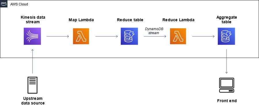
Overall, the data travels from the upstream data source, passes through the pipeline, lands in the DynamoDB aggregate table, and is read by a front end. For this post, we use a sample record generator that takes the role of the upstream data source (we refer to it as the producer). Generally speaking, you may have one or more data sources that are hosted on-premises, in AWS, or from a third-party. For simplicity, our CloudFormation template provides only one data source, hosted in the AWS Cloud. The producer generates random messages and ingests them into a Kinesis data stream. This data stream is defined to be the event source for a fleet of Lambda functions that we refer to as the map Lambda functions.
At each invocation, the map Lambda function picks up a batch of messages (up to 5,000) from the data stream, computes the aggregates over all the messages in the batch (based on the configured aggregation hierarchy), and writes the pre-aggregated data to the DynamoDB reduce table.
The partition key of this table is called MessageHash and is used to ensure that we don’t accidentally process any batch more than once. To do this, the map Lambda function calculates not only the aggregates, but also a SHA256 hash over the full list of records in the Lambda invocation event. This is the MessageHash that uniquely identifies each batch of messages. When persisting the results of the aggregation to the reduce table, we perform a conditional write of a single item, which contains the aggregates of the batch. The write is only run if the value of the partition key (the hash we described) hasn’t been seen before. This allows us to ensure we don’t process the same batch twice. However, with this architecture, there is still a small chance of individual messages being duplicated at the first stage of this pipeline, i.e., when the producer retries a message that has already been ingested up by the Kinesis data stream.
| If you’re interested in how this can be prevented, see Build a fault-tolerant, serverless data aggregation pipeline with exactly-once processing, where we go into more detail on deduplication and failure handling for serverless aggregation pipelines, and also discuss the relevant code snippets. |
Furthermore, the reduce table has DynamoDB Streams enabled: a DynamoDB stream is an ordered flow of information about changes to items in a DynamoDB table. When the stream is enabled on a table, DynamoDB captures all data modifications at the item level and sends updates into a stream that can be processed further.
The stream of the reduce table is defined as the event source for the reduce Lambda function. This Lambda function is invoked with a batch of items that were written into the reduce table (each item written in the reduce table is a reduced pre-aggregation of up to 5,000 risk messages, previously computed by the map function). A quick note on cost in this context: DynamoDB Streams is free to enable, but you incur charges when reading data from the stream using the SDKs. However, there’s no cost for reading from DynamoDB Streams when you connect it to a Lambda function, as we do with this specific architecture.
The reduce function performs the following operations:
- Compute the full aggregate over the batch of pre-aggregated items the function was invoked with.
- Update the values in the aggregate table using a single transactional write operation that increments all the current values with the results from the preceding step.
The reduce Lambda function is configured with a reserved concurrency of 1, which allows only a single instance of this function to be run at any time. This prevents race conditions and write conflicts that occur whenever multiple functions attempt to update the same rows in the aggregate table. For more information about concurrency, see Managing AWS Lambda Function Concurrency.
Finally, we also wrote a simple, Python-based front end that regularly polls the aggregated data table for updates and displays the results in your command line shell.
Throughput and capacity requirements
The producer generates random messages following the schema we described at rates of up to 50,000 messages per second and ingests them into the aggregation pipeline.
This architecture ensures consistency while maintaining horizontal scalability: if the data stream observes a high throughput, the pipeline automatically invokes a large number of instances of the map Lambda function. Let’s assume we have on average 100 map Lambda functions running concurrently, each pre-aggregating 500 risk messages with a runtime of 1,000 milliseconds and writing the results to the reduce table. The single active instance of the reduce function only needs to compute the sum over the 100 new items in this table every second and increment the total aggregates. In this example, the pipeline handles a total throughput of 50,000 messages per second with fairly low resource requirements of just around 100 concurrent function invocations and 100 DynamoDB write operations per second.
Evaluation
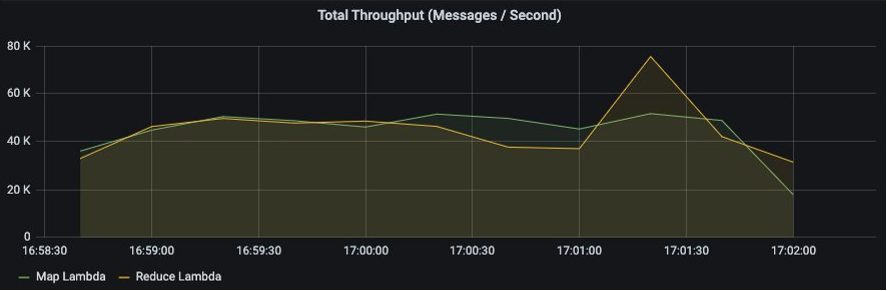
The following diagram shows the results of a test in which we ingested 10 million messages in around 200 seconds (the total throughput is computed as a rolling mean over 20 seconds). The horizontal axis shows the time, and the vertical axis is specified on the top of each of the following graphs.
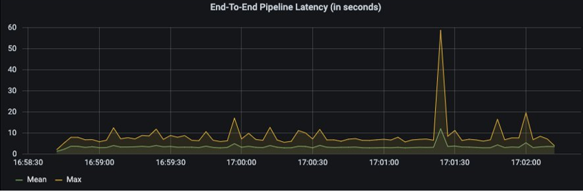
The total throughput is fairly constant at 50,000 messages per second, the mean end-to-end latency stays at 3–4 seconds for most of the test, with one spike at around 10 seconds, as shown in the following metrics.
You can run a pipeline with this architecture at a scale of 50,000 messages per second, 24 hours a day, 7 days a week for less than $3,000 USD per month in the US East (Ohio) Region.
The preceding graphs were produced using Grafana in conjunction with InfluxDB. Our source code contains a flag in the file Common/constants.py that you can set to true, in order to start sending data to InfluxDB, enabling the performance visualization with Grafana. If you want to do this, you also need to set up a Grafana instance with InfluxDB, for example using Amazon Managed Service for Grafana, and provide the IP of the instance, as well as the connection string for InfluxDB in the file Common/constants.py.
Security
At AWS, security is our top priority. The architecture outlined in this post inherits the security and compliance controls natively built into the AWS Cloud and integrated with Kinesis, Lambda, and DynamoDB.
When generally thinking about potential threats to a data aggregation pipeline like this, confidentiality, data integrity, and availability come to mind. In this section, we address how we’re using the different AWS services to mitigate each of these concerns.
Confidentiality
We want to ensure that only authorized parties can access the data in the pipeline. Therefore, we use the granular access controls offered by AWS Identity and Access Management (IAM) policies. Each of the Lambda functions in our architecture is only authorized to read from the previous stream component and write to next one. To outline this along a specific example, let’s look at an excerpt of the IAM policy that is attached to the map Lambda function in the CloudFormation templates:
The Lambda function is only authorized to perform the specific API calls that are necessary for the data flow in the pipeline.
In the CloudFormation templates that we provide in this post, both the upstream data source and the front end run in a single AWS Cloud9 instance. AWS Cloud9 is a cloud-based integrated development environment (IDE) that lets you write, run, and debug your code with just a browser. It includes a code editor, debugger, and terminal.
This instance uses the default approach of AWS managed temporary credentials. When the instance calls any AWS service, AWS Cloud9 checks to see if the calling AWS entity (for example, the IAM user) has the necessary permissions to perform the requested action. If the permission doesn’t exist or is explicitly denied, the request fails. Therefore, the authorization is based on the permissions of the IAM user accessing the AWS Cloud9 instance. For the pipeline to work as expected, you need to ensure that the IAM user has the necessary privileges.
Firstly, they need minimal permissions to run the upstream data source:
They also need minimal permissions to run the front end:
In both cases, you need to replace the placeholders <AWS_REGION>, <AWS_ACCOUNT_ID>, and <KINESIS_STREAM_NAME> or <AGGREGATE_TABLE_NAME> with their respective values.
Furthermore, we naturally want to ensure that the data is encrypted from end-to-end. The communication between all stages of the pipeline uses the secure HTTPS protocol, and both DynamoDB and Kinesis allow encryption at rest (also called server-side encryption) with the encryption keys managed by AWS Key Management Service (AWS KMS).
Kinesis Data Streams doesn’t have server-side encryption by default, so we enabled it in the provided CloudFormation templates. In contrast, all user data stored in DynamoDB is fully encrypted at rest by default. You can choose between different types of AWS KMS keys; for this post, we use AWS-owned keys for both Kinesis and DynamoDB.
Data integrity
The best practice of least privileges that we’ve outlined also helps ensure data integrity. Write permissions are strictly limited to the necessary components of the pipeline. Furthermore, data integrity rests on the ability of our pipeline to process the data consistently, namely to prevent duplicates as well as dropped messages. You can find more detail on the exactly-once processing semantics in Build a highly fault-tolerant, serverless data aggregation pipeline with exactly-once processing.
Availability
Finally, a concern that’s especially relevant for customers in highly regulated industries, like the banking industry that’s serving as an example for us, is availability. Downtimes of any business-relevant system can potentially be very costly, therefore we use fully managed, serverless AWS services, namely Kinesis, Lambda, and DynamoDB, with built-in fault tolerance and availability.
Explore the pipeline in your AWS account
You can easily deploy the architecture described in this post in your own AWS account using the provided CloudFormation template. The template deploys a pipeline that allows you to test and investigate serverless data aggregation. It comes with an AWS Cloud9 instance that can run the producer, as well as the front end.
Running the provided CloudFormation template in your own account may incur costs. Following the exact steps outlined in this post in any Region of your choice will incur charges of less than $1 USD, but be careful to clean up all of the resources after use.
To deploy the solution architecture, complete the following steps:
- Download the following CloudFormation template.
- Navigate to the AWS CloudFormation console in your preferred Region.
- Choose Create stack, then choose With new resources (standard).
- Choose Upload a template file and choose the file you downloaded.
- Choose Next.
- Enter a name for the stack, such as ServerlessAggregationStack.
- Choose Next.
- Leave all remaining defaults and choose Next.
- Select I acknowledge that AWS CloudFormation… and choose Create stack.
Stack creation takes 1–2 minutes. When it’s complete, we’re ready to run the pipeline.
- On the AWS Cloud9 console, locate the instance
StatelessDataProducer.
If you don’t see it, make sure you’re in the same Region that you used to create the CloudFormation stack.
- Choose Open IDE.
- Open a terminal and run the following commands to prepare the pipeline:
The pipeline is ready!
- Start the front end with the following code:
- Open an additional terminal and start the producer:
The data should start arriving in batches at the front end. You can confirm the accuracy of the aggregation by comparing the two sets of numbers. In rare cases, you may observe duplicates introduced due to retries in the pipeline, as described previously.
Before you run the producer again, you may want to reset the aggregation table displayed in the front end by running the following commands:
Clean up
Clean up your resources to prevent unexpected costs:
- On the AWS CloudFormation console, choose Stacks.
- Select the stack you created (
ServerlessAggregationStack). - Choose Delete.
- Confirm by choosing Delete stack.
You should see the status DELETE_IN_PROGRESS and after 1–2 minutes, the delete should be complete and the stack disappears from the list.
Conclusion
In this post, we introduced a serverless architecture for near real-time data aggregation based on Kinesis Data Streams, Lambda, and DynamoDB. This addresses a business problem faced by customers in various industries like manufacturing, retail, gaming, utilities, and financial services. Based on a specific example from the banking industry, we demonstrated that the pipeline can horizontally scale to handle up to 50,000 messages per second.
Although this solution shows great scalability, low latency, and cost-efficiency, there are still two limitations that we can improve further:
- The pipeline is stateless – Values of the individual trades aren’t preserved, which makes it impossible to modify trades that ran at an earlier stage.
- The pipeline isn’t designed to provide exactly-once processing semantics – Although we can ensure that any write to DynamoDB is idempotent (more details on this to follow), it’s not possible to identify duplicate messages in the Kinesis data stream (for example, due to producer retries), because we don’t keep track of the IDs of the messages that have been processed.
| If you’re interested in how to address these issues, we recommend to see Build a fault-tolerant, serverless data aggregation pipeline with exactly-once processing, where we introduce a slightly modified architecture that addresses these limitations. |
Both Lucas and Kirill are part of the of the Acceleration team within Global Financial Services, that aims to accelerate our customers’ cloud journey. If you’re interested in running a pipeline like this in production or if you have other questions to the team, you can contact them with an e-mail to gfs-acceleration-interest@amazon.com.
About the Authors
 Lucas Rettenmeier is a Solutions Architect based in Munich, Germany. His journey at AWS started in Business Development. After completing his M.Sc. in Physics at Heidelberg University with a focus on Machine Learning, he re-joined in 2020 as a Solutions Architect. He’s part of the Acceleration team within Global Financial Services, that aims to accelerate our customers’ cloud journey. Lucas is especially passionate about purpose-built databases and serverless technologies. Outside of work, he spends the majority of his time in nature either cycling, hiking, skiing, or trying something new.
 Kirill Bogdanov is a Senior Solutions Architect in the Amazon Web Services (AWS) for Global Financial Services. He provides cloud-native architecture designs and prototype implementations to build highly reliable, scalable, secure, and cost-efficient solutions ensuring the customers’ long-term business objectives and strategies. Kirill is a Ph.D. in Computer Science from KTH Royal Institute of Technology with expertise in distributed systems and High-Performance Computing (HPC). He has 12 years of experience in R&D, cloud migration, developing large-scale innovative solutions leveraging cloud technologies, and driving digital transformation.