Gaining insights into winning football strategies using machine learning

University of Illinois, Urbana Champaign (UIUC) has partnered with the Amazon Machine Learning Solutions Lab to help UIUC football coaches prepare for games more efficiently and improve their odds of winning.

Previously, coaches prepared for games by creating a game planning sheet that only featured types of plays for a certain down and distance, and where the team was on the field. As a result, the coaching staff might miss important scenarios and opportunities. Additionally, preparing a game planning sheet was a manual process, with new data for each game being entered into a template each week, which is time-consuming and not scalable.

To add more insights to the current call sheet templates and help coaches prepare for games better, the team combined UIUC’s deep expertise in college football and coaching with the machine learning (ML) capabilities of Amazon SageMaker to create a state-of-the-art ML model that predicts the result of UIUC’s football plays. In addition, UIUC coaches now have an auto-generated visual game planning sheet based on key features that the model recommends. This gives them more insights on their strategy for the game and reduces the time it takes to generate the visual game planning sheets from 2.5 hours to less than 30 seconds.

“The UIUC Athletic department collaborated with the Amazon ML Solutions Lab to harness the power of machine learning to derive data-driven insights on what features to include in our planning and preparation for our football games,” says Kingsley Osei-Asibey, Director of Analytics & Football Technology at UIUC. “By selecting AWS as our primary ML/AI platform, we got to work alongside the experts at the ML Solutions Lab to create new and interesting insights using Amazon SageMaker. Now, all the manual analysis of data from past games that took us hours is automated, and our Fighting Illini coaches can generate weekly visual game planning sheets against different opponents at the press of a button.”

This post looks at how the Amazon ML Solutions Lab used features related to the plays during a football game to predict the result of a play, and then used the XGBoost importance score feature and correlation analysis to recommend features for coaches to analyze.

We provide code snippets to show you how we used the Amazon SageMaker XGBoost library to generate feature importance scores.

Data and model

We used UIUC’s game data from the 2018–2019 college football season, covering 24 features including in-game statistics, location of the play, UIUC’s strategies, and their opponent’s play types. We used those features to train an XGBoost model to predict if an offensive play will result in a win or loss. The UIUC coaches decided whether it’s a win or loss for a play based on different situations.

We then used the feature importance scores to select key features. We used the model for feature-selection purposes to recommend important scenarios represented by features. We selected XGBoost because it performs well on features with complex distributions, and it outputs feature importance scores to help us with feature selection and model interpretation.

The main goal was to generate game planning sheets for football coaches to use in games to give them an edge. We used the features from a well performant ML model trained to classify successful and unsuccessful plays to inform coaches and generate game planning sheets.

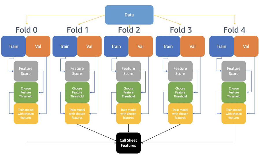
The following diagram summarizes the modeling steps taken to generate the ML-based features for the game planning sheet.

The rows are shuffled and split into five non-overlapping folds, which are then further split into training and validation sets. The training sets of each fold are balanced using the Synthetic Minority Oversampling Technique (SMOTE) algorithm.

Each fold includes the following steps:

1. Calculate a new feature score:
   1. Train an XGBoost model on the balanced training data set and extract the feature importances feat_i.
   2. Compute the Pearson’s correlation of the features and label in the balanced training dataset corr_i.
   3. Compute a new feature score as the product of absolute correlation and feature importance feature_score_i = feat_i * abs(corr_i).
2. Sort the features based on the feat_score.
3. Train multiple XGBoost models using the top 5 features, top 10 features, and so on, and evaluate validation balanced accuracy for each model.
4. Choose the best-performing model.

After we trained models from each of the five folds, we merged the important features. A feature is selected for the game planning sheet if it appears in the top 10 features (ranked by feature importance score) of at least three folds.

Calculating the new feature score

In the previous section, we described the construction of a new feature score. This new feature score incorporates the feature importance from a non-linear XGBoost model, as well as direct linear correlation. The purpose of this new feature score is to select features that are relevant to winning or losing a play. A feature with a high feature score has high XGBoost feature importance and high linear correlation with the label, making it a relevant feature for game planning sheets.

In this section, we dive deeper into the construction of the new feature score with code snippets. The feature score is a combination of feature importance from a trained XGBoost model and linear correlation of the features and the label.

First, we train an XGBoost model using Amazon SageMaker built-in algorithms. Amazon SageMaker is a fully managed service that provides every developer and data scientist with the ability to build, train, and deploy ML models quickly. Amazon SageMaker provides several built-in algorithms (such as XGBoost) for a variety of problem types.

This trained XGBoost model provides a first look into which features are important to the UIUC football team winning a play. See the following code:

from sagemaker.amazon.amazon_estimator import get_image_uri
container = get_image_uri(region, "xgboost", "0.90-1")

hyperparameters = {
    "max_depth":"7",
    "eta":"0.01",
    "gamma":"3",
    "min_child_weight":"6",
    "subsample":"0.6",
    "silent":"0",
    "objective":"binary:logistic",
    "num_round":"330"
}

instance_type = 'ml.m5.2xlarge'
output_path = "s3://{}/{}/{}/output".format(bucket, "model", "xgboost")

job_name = "xgboost-".format(i+1) + time.strftime("%Y-%m-%d-%H-%M-%S", time.gmtime())

estimator = sagemaker.estimator.Estimator(
    container, 
    role, 
    hyperparameters=hyperparameters,
    train_instance_count=1, 
    train_instance_type=instance_type, 
    train_volume_size=5,
    output_path=output_path, 
    sagemaker_session=sagemaker.Session()
)

train_input = sagemaker.s3_input(
    s3_data="s3://{}/{}/{}".format(bucket, "train", "balanced_train_data.csv"), 
    content_type='csv'
)
estimator.fit({"train": train_input}, job_name=job_name)

Amazon SageMaker stores the model object in the specified Amazon Simple Storage Service (Amazon S3) bucket. To calculate the feature score, we need to download model.tar.gz from Amazon S3 to our Amazon SageMaker notebook instance. See the following code:

model_path = "s3://{}/{}/{}/output/{}".format(
    bucket, "model", "xgboost",
    "xgboost-2019-06-16-09-56-39-854/output/model.tar.gz"
)

fs = s3fs.S3FileSystem()

with fs.open(model_path, "rb") as f:
    with tarfile.open(fileobj=f, mode="r") as tar_f:
        with tar_f.extractfile("xgboost-model") as extracted_f:
            xgbooster = pickle.load(extracted_f)

Finally, we calculate the new feature score as feature_score_i = feat_i * abs(corr_i). We use the absolute value of the correlation because our goal is to find features that are relevant to winning or losing a play, and a highly negative correlation indicates a strong linear relationship between the feature and the UIUC football team losing the play. See the following code:

#the xgbooster object replaces the original feature names with 'f0,...f'
#here we create a mapping to obtain the original feature names
feature_name_map = dict(zip([f"f{i}" for i in range(len(feature_names))], feature_names))

features_importance_df = pd.DataFrame([xgbooster.get_fscore()], index=["weight"]).T
features_importance_df["normalized_weight"] = features_importance_df["weight"]/features_importance_df["weight"].sum()
feature_importances_df["feature_name"] = feature_importances_df.index.map(feature_name_map)

correlation_df = pd.DataFrame(balanced_train_data_df[FEATURES].corr()[LABEL])
correlation_df["absolute_corr"] = correlation_df[LABEL].abs()

feature_score_df = pd.merge(
    features_importance_df, correlation_df.reset_index(), 
    left_on="feature_name", right_on="index"
)

feature_score_df["feature_score"] = feature_score_df["absolute_corr"] * feature_score_df["normalized_weight"]

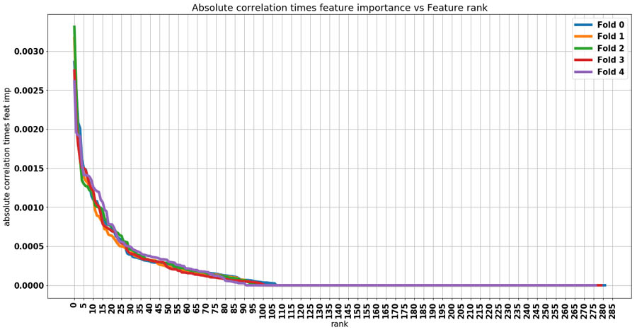
The following graph shows a plot of feature_score vs.rank for each fold. High values on the y-axis indicate that the feature was important for the XGBoost model and has high correlation with winning or losing a play. The key takeaway from this plot is additional features after feature number 105 don’t add any new information, and the optimum number of features to use lies between 0–105.

Evaluating the model

We performed five-fold cross-validation on the XGBoost model, and compared it to three baseline models: a model predicting every sample as lost, a model predicting every sample as win, and a random model assigning win or loss with a 50/50 chance.

Because the dataset is imbalanced with 56% of the plays labeled as lost and 44% as won, we used the weighted accuracy metrics considering the class weights when comparing our model to the naïve baselines. The weighted accuracy for all three naïve baselines is 50%, and average weighted accuracy of the XGBoost is 65.2% across five folds, which shows that our model has 15% improvement compared to the baselines.

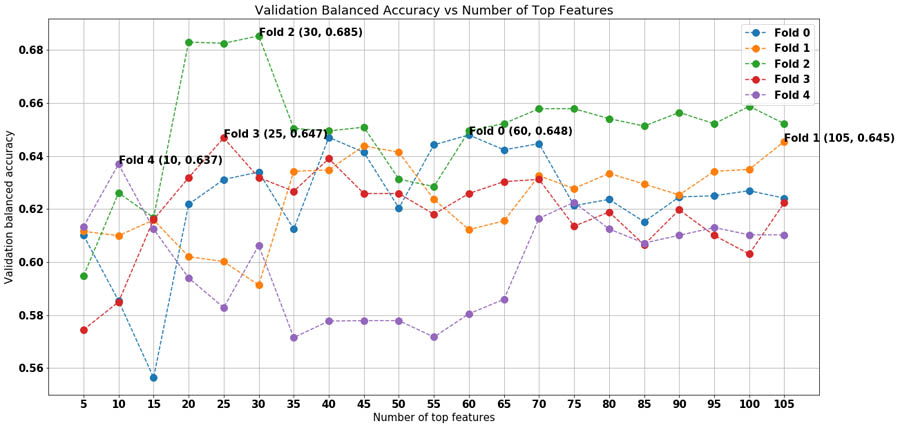
The following plot shows validation balanced accuracy vs. the number of top features for each fold. For each data point, an XGBoost model is trained using the top n features, where n is the value on the x-axis, and evaluated on the fold’s validation dataset to obtain the validation balanced accuracy. The top performing model for each is annotated in the plot. For example, Fold 0’s best-performing model uses the top 60 features (as determined in the preceding plot), which has a validation balanced accuracy of 64.8%. Features ranked above 105 aren’t evaluated because the previous plot shows that features ranked above 105 contribute little information.

The following table summarizes the results of the procedure we outlined. For each fold, the balanced accuracy performance improves after performing feature selection, with an average increase of 3.2%.

To further improve the models, we used Amazon SageMaker automated model tuning for hyperparameter optimization. We used the best features identified in the preceding step for each fold, and performed 20 iterations of Bayesian optimization on each fold.

Feature selection and game planning sheet recommendation across five folds

The end goal is to create a new game planning sheet using features derived from the XGBoost models. A high-performing model indicates that the extracted features are relevant to winning a play. The output of the training stage results in an XGBoost model for each fold. A feature is selected for the game planning sheet if it appears in the top 10 features (ranked by feature importance score) of at least three folds.

After reviewing these features with the UIUC coaching staff, the coaches designed new game planning sheets to analyze the best play types based on how their opponent would be playing defense. These additional features will help the coaches prepare more scenarios before the games start, and players can react faster and more accurately against opponents.

Summary

UIUC football coaches partnered with the Amazon ML Solutions Lab and created an ML model to gain more insights on their performance and strategies. This solution also saves the coaches’ time when preparing for a game; instead of manually analyzing the best plays to call under different situations, coaches can automate this process using the features the ML model recommends.

This model is customized for UIUC’s football team and their opponents, and will help UIUC’s coaches prepare for more scenarios in upcoming seasons. Additionally, it will help players react correctly and quickly to game situations.

If you’d like help accelerating the use of ML in your products and services, please contact the Amazon ML Solutions Lab program.

About the Authors

 Ninad Kulkarni is a Data Scientist in the Amazon Machine Learning Solutions Lab. He helps customers adopt ML and AI by building solutions to address their business problems. Most recently, he has built predictive models for sports and automotive customers.

Daliana Zhen Liu is a Data Scientist in the Amazon Machine Learning Solutions Lab. She has built ML models to help customers accelerate their business in sports, media and education. She is passionate about introducing data science to more people.

Tianyu Zhang is a Data Scientist in the Amazon Machine Learning Solutions Lab. He helps customers solve business problems by applying ML and AI techniques. Most recently, he has built NLP model and predictive model for procurement and sports.