Artificial Intelligence
How Light & Wonder built a predictive maintenance solution for gaming machines on AWS
This post is co-written with Aruna Abeyakoon and Denisse Colin from Light and Wonder (L&W).
Headquartered in Las Vegas, Light & Wonder, Inc. is the leading cross-platform global game company that provides gambling products and services. Working with AWS, Light & Wonder recently developed an industry-first secure solution, Light & Wonder Connect (LnW Connect), to stream telemetry and machine health data from roughly half a million electronic gaming machines distributed across its casino customer base globally when LnW Connect reaches its full potential. Over 500 machine events are monitored in near-real time to give a full picture of machine conditions and their operating environments. Utilizing data streamed through LnW Connect, L&W aims to create better gaming experience for their end-users as well as bring more value to their casino customers.
Light & Wonder teamed up with the Amazon ML Solutions Lab to use events data streamed from LnW Connect to enable machine learning (ML)-powered predictive maintenance for slot machines. Predictive maintenance is a common ML use case for businesses with physical equipment or machinery assets. With predictive maintenance, L&W can get advanced warning of machine breakdowns and proactively dispatch a service team to inspect the issue. This will reduce machine downtime and avoid significant revenue loss for casinos. With no remote diagnostic system in place, issue resolution by the Light & Wonder service team on the casino floor can be costly and inefficient, while severely degrading the customer gaming experience.
The nature of the project is highly exploratory—this is the first attempt at predictive maintenance in the gaming industry. The Amazon ML Solutions Lab and L&W team embarked on an end-to-end journey from formulating the ML problem and defining the evaluation metrics, to delivering a high-quality solution. The final ML model combines CNN and Transformer, which are the state-of-the-art neural network architectures for modeling sequential machine log data. The post presents a detailed description of this journey, and we hope you will enjoy it as much as we do!
In this post, we discuss the following:
- How we formulated the predictive maintenance problem as an ML problem with a set of appropriate metrics for evaluation
- How we prepared data for training and testing
- Data preprocessing and feature engineering techniques we employed to obtain performant models
- Performing a hyperparameter tuning step with Amazon SageMaker Automatic Model Tuning
- Comparisons between the baseline model and the final CNN+Transformer model
- Additional techniques we used to improve model performance, such as ensembling
Background
In this section, we discuss the issues that necessitated this solution.
Dataset
Slot machine environments are highly regulated and are deployed in an air-gapped environment. In LnW Connect, an encryption process was designed to provide a secure and reliable mechanism for the data to be brought into an AWS data lake for predictive modeling. The aggregated files are encrypted and the decryption key is only available in AWS Key Management Service (AWS KMS). A cellular-based private network into AWS is set up through which the files were uploaded into Amazon Simple Storage Service (Amazon S3).
LnW Connect streams a wide range of machine events, such as start of game, end of game, and more. The system collects over 500 different types of events. As shown in the following
, each event is recorded along with a timestamp of when it happened and the ID of the machine recording the event. LnW Connect also records when a machine enters a non-playable state, and it will be marked as a machine failure or breakdown if it doesn’t recover to a playable state within a sufficiently short time span.
| Machine ID | Event Type ID | Timestamp |
|---|---|---|
| 0 | E1 | 2022-01-01 00:17:24 |
| 0 | E3 | 2022-01-01 00:17:29 |
| 1000 | E4 | 2022-01-01 00:17:33 |
| 114 | E234 | 2022-01-01 00:17:34 |
| 222 | E100 | 2022-01-01 00:17:37 |
In addition to dynamic machine events, static metadata about each machine is also available. This includes information such as machine unique identifier, cabinet type, location, operating system, software version, game theme, and more, as shown in the following table. (All the names in the table are anonymized to protect customer information.)
| Machine ID | Cabinet Type | OS | Location | Game Theme |
|---|---|---|---|---|
| 276 | A | OS_Ver0 | AA Resort & Casino | StormMaiden |
| 167 | B | OS_Ver1 | BB Casino, Resort & Spa | UHMLIndia |
| 13 | C | OS_Ver0 | CC Casino & Hotel | TerrificTiger |
| 307 | D | OS_Ver0 | DD Casino Resort | NeptunesRealm |
| 70 | E | OS_Ver0 | EE Resort & Casino | RLPMealTicket |
Problem definition
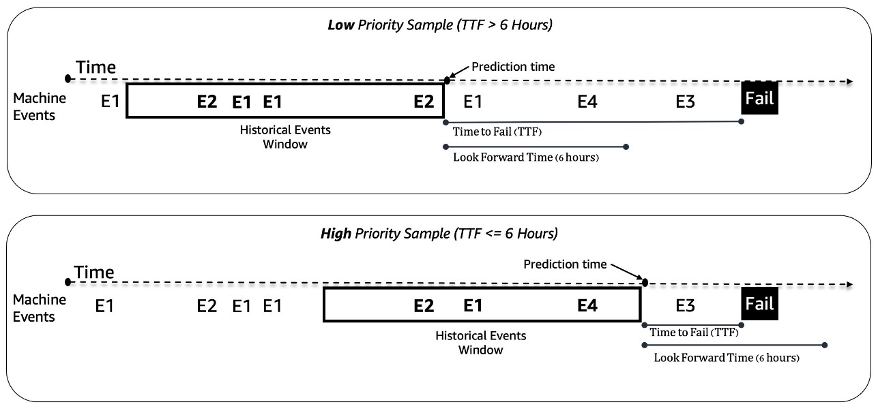
We treat the predictive maintenance problem for slot machines as a binary classification problem. The ML model takes in the historical sequence of machine events and other metadata and predicts whether a machine will encounter a failure in a 6-hour future time window. If a machine will break down within 6 hours, it is deemed a high-priority machine for maintenance. Otherwise, it is low priority. The following figure gives examples of low-priority (top) and high-priority (bottom) samples. We use a fixed-length look-back time window to collect historical machine event data for prediction. Experiments show that longer look-back time windows improve model performance significantly (more details later in this post).
Modeling challenges
We faced a couple of challenges solving this problem:
- We have a huge amount event logs that contain around 50 million events a month (from approximately 1,000 game samples). Careful optimization is needed in the data extraction and preprocessing stage.
- Event sequence modeling was challenging due to the extremely uneven distribution of events over time. A 3-hour window can contain anywhere from tens to thousands of events.
- Machines are in a good state most of the time and the high-priority maintenance is a rare class, which introduced a class imbalance issue.
- New machines are added continuously to the system, so we had to make sure our model can handle prediction on new machines that have never been seen in training.
Data preprocessing and feature engineering
In this section, we discuss our methods for data preparation and feature engineering.
Feature engineering
Slot machine feeds are streams of unequally spaced time series events; for example, the number of events in a 3-hour window can range from tens to thousands. To handle this imbalance, we used event frequencies instead of the raw sequence data. A straightforward approach is aggregating the event frequency for the entire look-back window and feeding it into the model. However, when using this representation, the temporal information is lost, and the order of events is not preserved. We instead used temporal binning by dividing the time window into N equal sub-windows and calculating the event frequencies in each. The final features of a time window are the concatenation of all its sub-window features. Increasing the number of bins preserves more temporal information. The following figure illustrates temporal binning on a sample window.

First, the sample time window is split into two equal sub-windows (bins); we used only two bins here for simplicity for illustration. Then, the counts of the events E1, E2, E3, and E4 are calculated in each bin. Lastly, they are concatenated and used as features.
Along with the event frequency-based features, we used machine-specific features like software version, cabinet type, game theme, and game version. Additionally, we added features related to the timestamps to capture the seasonality, such as hour of the day and day of the week.
Data preparation
To extract data efficiently for training and testing, we utilize Amazon Athena and the AWS Glue Data Catalog. The events data is stored in Amazon S3 in Parquet format and partitioned according to day/month/hour. This facilitates efficient extraction of data samples within a specified time window. We use data from all machines in the latest month for testing and the rest of the data for training, which helps avoid potential data leakage.
ML methodology and model training
In this section, we discuss our baseline model with AutoGluon and how we built a customized neural network with SageMaker automatic model tuning.
Building a baseline model with AutoGluon
With any ML use case, it’s important to establish a baseline model to be used for comparison and iteration. We used AutoGluon to explore several classic ML algorithms. AutoGluon is easy-to-use AutoML tool that uses automatic data processing, hyperparameter tuning, and model ensemble. The best baseline was achieved with a weighted ensemble of gradient boosted decision tree models. The ease of use of AutoGluon helped us in the discovery stage to navigate quickly and efficiently through a wide range of possible data and ML modeling directions.
Building and tuning a customized neural network model with SageMaker automatic model tuning
After experimenting with different neural networks architectures, we built a customized deep learning model for predictive maintenance. Our model surpassed the AutoGluon baseline model by 121% in recall at 80% precision. The final model ingests historical machine event sequence data, time features such as hour of the day, and static machine metadata. We utilize SageMaker automatic model tuning jobs to search for the best hyperparameters and model architectures.
The following figure shows the model architecture. We first normalize the binned event sequence data by average frequencies of each event in the training set to remove the overwhelming effect of high-frequency events (start of game, end of game, and so on). The embeddings for individual events are learnable, while the temporal feature embeddings (day of the week, hour of the day) are extracted using the package GluonTS. Then we concatenate the event sequence data with the temporal feature embeddings as the input to the model. The model consists of the following layers:
- Convolutional layers (CNN) – Each CNN layer consists of two 1-dimensional convolutional operations with residual connections. The output of each CNN layer has the same sequence length as the input to allow for easy stacking with other modules. The total number of CNN layers is a tunable hyperparameter.
- Transformer encoder layers (TRANS) – The output of the CNN layers is fed together with the positional encoding to a multi-head self-attention structure. We use TRANS to directly capture temporal dependencies instead of using recurrent neural networks. Here, binning of the raw sequence data (reducing length from thousands to hundreds) helps alleviate the GPU memory bottlenecks, while keeping the chronological information to a tunable extent (the number of the bins is a tunable hyperparameter).
- Aggregation layers (AGG) – The final layer combines the metadata information (game theme type, cabinet type, locations) to produce the priority level probability prediction. It consists of several pooling layers and fully connected layers for incremental dimension reduction. The multi-hot embeddings of metadata are also learnable, and don’t go through CNN and TRANS layers because they don’t contain sequential information.

We use the cross-entropy loss with class weights as tunable hyperparameters to adjust for the class imbalance issue. In addition, the numbers of CNN and TRANS layers are crucial hyperparameters with the possible values of 0, which means specific layers may not always exist in the model architecture. This way, we have a unified framework where the model architectures are searched along with other usual hyperparameters.
We utilize SageMaker automatic model tuning, also known as hyperparameter optimization (HPO), to efficiently explore model variations and the large search space of all hyperparameters. Automatic model tuning receives the customized algorithm, training data, and hyperparameter search space configurations, and searches for best hyperparameters using different strategies such as Bayesian, Hyperband, and more with multiple GPU instances in parallel. After evaluating on a hold-out validation set, we obtained the best model architecture with two layers of CNN, one layer of TRANS with four heads, and an AGG layer.
We used the following hyperparameter ranges to search for the best model architecture:
To further improve model accuracy and reduce model variance, we trained the model with multiple independent random weight initializations, and aggregated the result with mean values as the final probability prediction. There is a trade-off between more computing resources and better model performance, and we observed that 5–10 should be a reasonable number in the current use case (results shown later in this post).
Model performance results
In this section, we present the model performance evaluation metrics and results.
Evaluation metrics
Precision is very important for this predictive maintenance use case. Low precision means reporting more false maintenance calls, which drives costs up through unnecessary maintenance. Because average precision (AP) doesn’t fully align with the high precision objective, we introduced a new metric named average recall at high precisions (ARHP). ARHP is equal to the average of recalls at 60%, 70%, and 80% precision points. We also used precision at top K% (K=1, 10), AUPR, and AUROC as additional metrics.
Results
The following table summarizes the results using the baseline and the customized neural network models, with 7/1/2022 as the train/test split point. Experiments show that increasing the window length and sample data size both improve the model performance, because they contain more historical information to help with the prediction. Regardless of the data settings, the neural network model outperforms AutoGluon in all metrics. For example, recall at the fixed 80% precision is increased by 121%, which enables you to quickly identify more malfunctioned machines if using the neural network model.
| Model | Window length/Data size | AUROC | AUPR | ARHP | Recall@Prec0.6 | Recall@Prec0.7 | Recall@Prec0.8 | Prec@top1% | Prec@top10% |
|---|---|---|---|---|---|---|---|---|---|
| AutoGluon baseline | 12H/500k | 66.5 | 36.1 | 9.5 | 12.7 | 9.3 | 6.5 | 85 | 42 |
| Neural Network | 12H/500k | 74.7 | 46.5 | 18.5 | 25 | 18.1 | 12.3 | 89 | 55 |
| AutoGluon baseline | 48H/1mm | 70.2 | 44.9 | 18.8 | 26.5 | 18.4 | 11.5 | 92 | 55 |
| Neural Network | 48H/1mm | 75.2 | 53.1 | 32.4 | 39.3 | 32.6 | 25.4 | 94 | 65 |
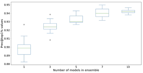
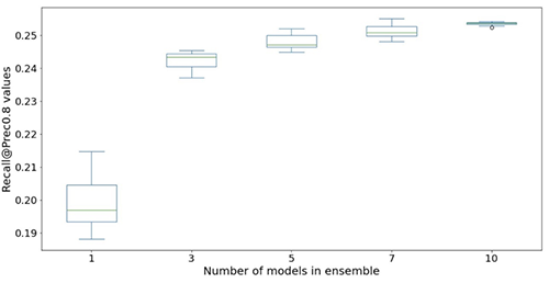
The following figures illustrate the effect of using ensembles to boost the neural network model performance. All the evaluation metrics shown on the x-axis are improved, with higher mean (more accurate) and lower variance (more stable). Each box-plot is from 12 repeated experiments, from no ensembles to 10 models in ensembles (x-axis). Similar trends persist in all metrics besides the Prec@top1% and Recall@Prec80% shown.
After factoring in the computational cost, we observe that using 5–10 models in ensembles is suitable for Light & Wonder datasets.
Conclusion
Our collaboration has resulted in the creation of a groundbreaking predictive maintenance solution for the gaming industry, as well as a reusable framework that could be utilized in a variety of predictive maintenance scenarios. The adoption of AWS technologies such as SageMaker automatic model tuning facilitates Light & Wonder to navigate new opportunities using near-real-time data streams. Light & Wonder is starting the deployment on AWS.
If you would like help accelerating the use of ML in your products and services, please contact the Amazon ML Solutions Lab program.
About the authors
 Aruna Abeyakoon is the Senior Director of Data Science & Analytics at Light & Wonder Land-based Gaming Division. Aruna leads the industry-first Light & Wonder Connect initiative and supports both casino partners and internal stakeholders with consumer behavior and product insights to make better games, optimize product offerings, manage assets, and health monitoring & predictive maintenance.
 Denisse Colin is a Senior Data Science Manager at Light & Wonder, a leading cross-platform global game company. She is a member of the Gaming Data & Analytics team helping develop innovative solutions to improve product performance and customers’ experiences through Light & Wonder Connect.
 Tesfagabir Meharizghi is a Data Scientist at the Amazon ML Solutions Lab where he helps AWS customers across various industries such as gaming, healthcare and life sciences, manufacturing, automotive, and sports and media, accelerate their use of machine learning and AWS cloud services to solve their business challenges.
 Mohamad Aljazaery is an applied scientist at Amazon ML Solutions Lab. He helps AWS customers identify and build ML solutions to address their business challenges in areas such as logistics, personalization and recommendations, computer vision, fraud prevention, forecasting and supply chain optimization.
 Yawei Wang is an Applied Scientist at the Amazon ML Solution Lab. He helps AWS business partners identify and build ML solutions to address their organization’s business challenges in a real-world scenario.
 Yun Zhou is an Applied Scientist at the Amazon ML Solutions Lab, where he helps with research and development to ensure the success of AWS customers. He works on pioneering solutions for various industries using statistical modeling and machine learning techniques. His interest includes generative models and sequential data modeling.
 Panpan Xu is a Applied Science Manager with the Amazon ML Solutions Lab at AWS. She is working on research and development of Machine Learning algorithms for high-impact customer applications in a variety of industrial verticals to accelerate their AI and cloud adoption. Her research interest includes model interpretability, causal analysis, human-in-the-loop AI and interactive data visualization.
 Raj Salvaji leads Solutions Architecture in the Hospitality segment at AWS. He works with hospitality customers by providing strategic guidance, technical expertise to create solutions to complex business challenges. He draws on 25 years of experience in multiple engineering roles across Hospitality, Finance and Automotive industries.
 Shane Rai is a Principal ML Strategist with the Amazon ML Solutions Lab at AWS. He works with customers across a diverse spectrum of industries to solve their most pressing and innovative business needs using AWS’s breadth of cloud-based AI/ML services.