Train and host a computer vision model for tampering detection on Amazon SageMaker: Part 2

In the first part of this three-part series, we presented a solution that demonstrates how you can automate detecting document tampering and fraud at scale using AWS AI and machine learning (ML) services for a mortgage underwriting use case.

In this post, we present an approach to develop a deep learning-based computer vision model to detect and highlight forged images in mortgage underwriting. We provide guidance on building, training, and deploying deep learning networks on Amazon SageMaker.

In Part 3, we demonstrate how to implement the solution on Amazon Fraud Detector.

Solution overview

To meet the objective of detecting document tampering in mortgage underwriting, we employ a computer vision model hosted on SageMaker for our image forgery detection solution. This model receives a testing image as input and generates a likelihood prediction of forgery as its output. The network architecture is as depicted in the following diagram.

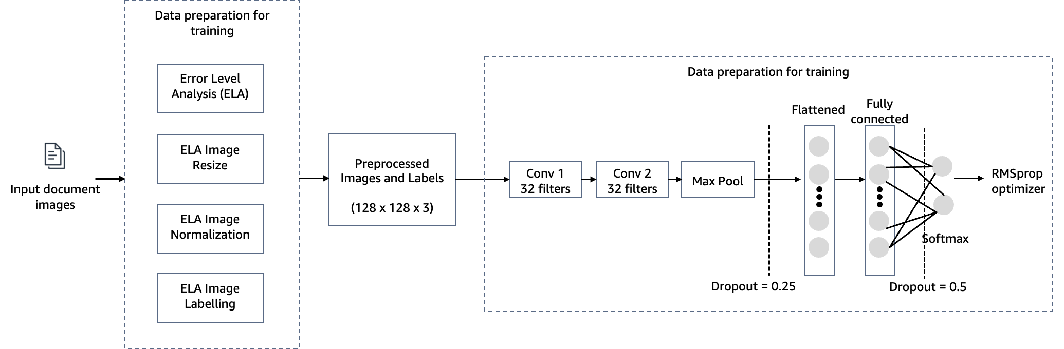
Tampering detection model architecture

Image forgery mainly involves four techniques: splicing, copy-move, removal, and enhancement. Depending on the characteristics of the forgery, different clues can be used as the foundation for detection and localization. These clues include JPEG compression artifacts, edge inconsistencies, noise patterns, color consistency, visual similarity, EXIF consistency, and camera model.

Given the expansive realm of image forgery detection, we use the Error Level Analysis (ELA) algorithm as an illustrative method for detecting forgeries. We selected the ELA technique for this post for the following reasons:

It is quicker to implement and can easily catch tampering of images.
It works by analyzing the compression levels of different parts of an image. This allows it to detect inconsistencies that may indicate tampering—for example, if one area was copied and pasted from another image that had been saved at a different compression level.
It is good at detecting more subtle or seamless tampering that may be hard to spot with the naked eye. Even small changes to an image can introduce detectable compression anomalies.
It doesn’t rely on having the original unmodified image for comparison. ELA can identify tampering signs within only the questioned image itself. Other techniques often require the unmodified original to compare against.
It is a lightweight technique that only relies on analyzing compression artifacts in the digital image data. It doesn’t depend on specialized hardware or forensics expertise. This makes ELA accessible as a first-pass analysis tool.
The output ELA image can clearly highlight differences in compression levels, making tampered areas visibly obvious. This allows even a non-expert to recognize signs of possible manipulation.
It works on many image types (such as JPEG, PNG, and GIF) and requires only the image itself to analyze. Other forensic techniques may be more restricted in formats or original image requirements.

However, in real-world scenarios where you may have a combination of input documents (JPEG, PNG, GIF, TIFF, PDF), we recommend employing ELA in conjunction with various other methods, such as detecting inconsistencies in edges, noise patterns, color uniformity, EXIF data consistency, camera model identification, and font uniformity. We aim to update the code for this post with additional forgery detection techniques.

ELA’s underlying premise assumes that the input images are in JPEG format, known for its lossy compression. Nevertheless, the method can still be effective even if the input images were originally in a lossless format (such as PNG, GIF, or BMP) and later converted to JPEG during the tampering process. When ELA is applied to original lossless formats, it typically indicates consistent image quality without any deterioration, rendering it challenging to pinpoint altered areas. In JPEG images, the expected norm is for the entire picture to exhibit similar compression levels. However, if a particular section within the image displays a markedly different error level, it often suggests a digital alteration has been made.

ELA highlights differences in the JPEG compression rate. Regions with uniform coloring will likely have a lower ELA result (for example, a darker color compared to high-contrast edges). The things to look for to identify tampering or modification include the following:

Similar edges should have similar brightness in the ELA result. All high-contrast edges should look similar to each other, and all low-contrast edges should look similar. With an original photo, low-contrast edges should be almost as bright as high-contrast edges.
Similar textures should have similar coloring under ELA. Areas with more surface detail, such as a close-up of a basketball, will likely have a higher ELA result than a smooth surface.
Regardless of the actual color of the surface, all flat surfaces should have about the same coloring under ELA.

JPEG images use a lossy compression system. Each re-encoding (resave) of the image adds more quality loss to the image. Specifically, the JPEG algorithm operates on an 8×8 pixel grid. Each 8×8 square is compressed independently. If the image is completely unmodified, then all 8×8 squares should have similar error potentials. If the image is unmodified and resaved, then every square should degrade at approximately the same rate.

ELA saves the image at a specified JPEG quality level. This resave introduces a known amount of errors across the entire image. The resaved image is then compared against the original image. If an image is modified, then every 8×8 square that was touched by the modification should be at a higher error potential than the rest of the image.

The results from ELA are directly dependent on the image quality. You may want to know if something was added, but if the picture is copied multiple times, then ELA may only permit detecting the resaves. Try to find the best quality version of the picture.

With training and practice, ELA can also learn to identify image scaling, quality, cropping, and resave transformations. For example, if a non-JPEG image contains visible grid lines (1 pixel wide in 8×8 squares), then it means the picture started as a JPEG and was converted to non-JPEG format (such as PNG). If some areas of the picture lack grid lines or the grid lines shift, then it denotes a splice or drawn portion in the non-JPEG image.

In the following sections, we demonstrate the steps for configuring, training, and deploying the computer vision model.

Prerequisites

To follow along with this post, complete the following prerequisites:

Have an AWS account.
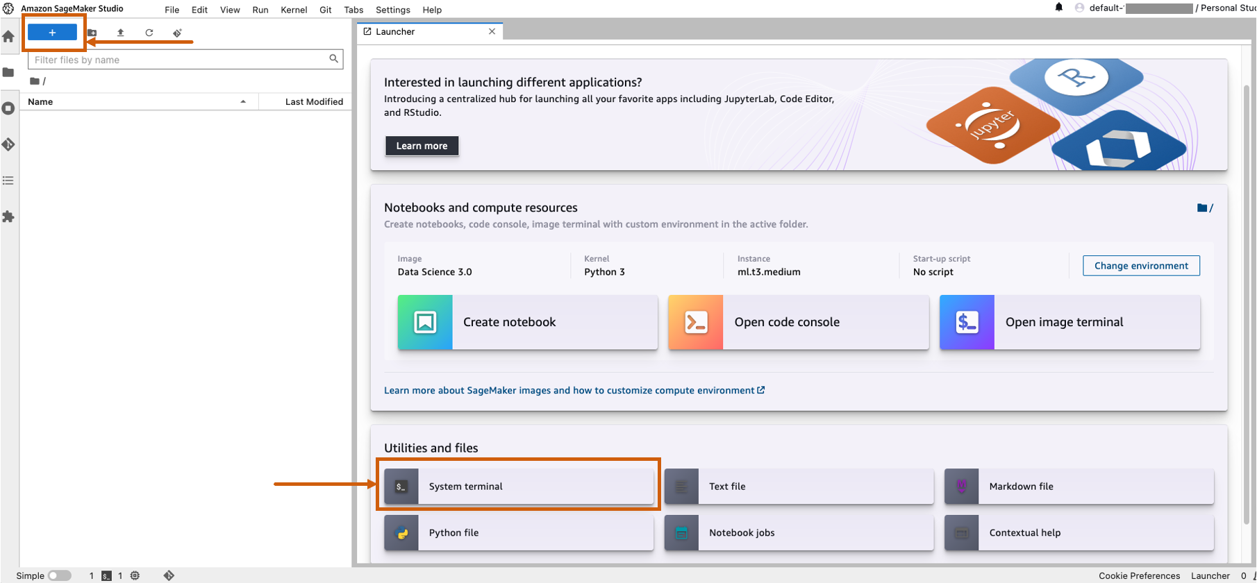
Set up Amazon SageMaker Studio. You can swiftly initiate SageMaker Studio using default presets, facilitating a rapid launch. For more information, refer to Amazon SageMaker simplifies the Amazon SageMaker Studio setup for individual users.
Open SageMaker Studio and launch a system terminal.
Run the following command in the terminal:
git clone https://github.com/aws-samples/document-tampering-detection.git
The total cost of running SageMaker Studio for one user and the configurations of the notebook environment is $7.314 USD per hour.

Set up the model training notebook

Complete the following steps to set up your training notebook:

Open the tampering_detection_training.ipynb file from the document-tampering-detection directory.
Set up the notebook environment with the image TensorFlow 2.6 Python 3.8 CPU or GPU Optimized.
You may run into issue of insufficient availability or hit the quota limit for GPU instances within your AWS account when selecting GPU optimized instances. To increase the quota, visit the Service Quotas console and increase the service limit for the specific instance type you need. You can also use a CPU optimized notebook environment in such cases.
For Kernel, choose Python3.
For Instance type, choose ml.m5d.24xlarge or any other large instance.

We selected a larger instance type to reduce the training time of the model. With an ml.m5d.24xlarge notebook environment, the cost per hour is $7.258 USD per hour.

Run the training notebook

Run each cell in the notebook tampering_detection_training.ipynb in order. We discuss some cells in more detail in the following sections.

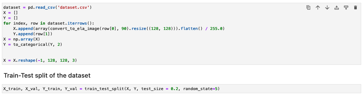
Prepare the dataset with a list of original and tampered images

Before you run the following cell in the notebook, prepare a dataset of original and tampered documents based on your specific business requirements. For this post, we use a sample dataset of tampered paystubs, and bank statements. The dataset is available within the images directory of the GitHub repository.

Prepare dataset

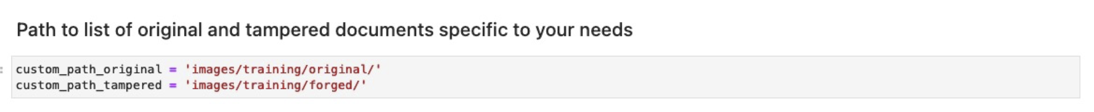
The notebook reads the original and tampered images from the images/training directory.

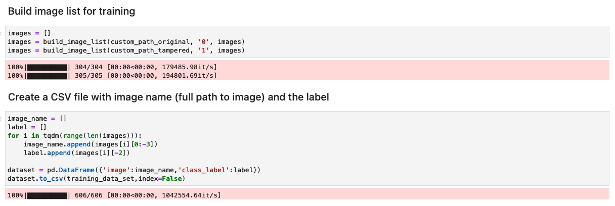
The dataset for training is created using a CSV file with two columns: the path to the image file and the label for the image (0 for original image and 1 for tampered image).

Label dataset

Process the dataset by generating the ELA results of each training image

In this step, we generate the ELA result (at 90% quality) of the input training image. The function convert_to_ela_image takes two parameters: path, which is the path to an image file, and quality, representing the quality parameter for JPEG compression. The function performs the following steps:

Convert the image to RGB format and resave the image as a JPEG file with the specified quality under the name tempresaved.jpg.
Compute the difference between the original image and the resaved JPEG image (ELA) to determine the maximum difference in pixel values between the original and resaved images.
Calculate a scale factor based on the maximum difference to adjust the brightness of the ELA image.
Enhance the brightness of the ELA image using the calculated scale factor.
Resize the ELA result to 128x128x3, where 3 represents the number of channels to reduce the input size for training.
Return the ELA image.

In lossy image formats such as JPEG, the initial saving process leads to considerable color loss. However, when the image is loaded and subsequently re-encoded in the same lossy format, there’s generally less added color degradation. ELA outcomes emphasize the image areas most susceptible to color degradation upon resaving. Generally, alterations appear prominently in regions exhibiting higher potential for degradation compared to the rest of the image.

Next, the images are processed into a NumPy array for training. We then split the input dataset randomly into training and test or validation data (80/20). You can ignore any warnings when running these cells.

Convert to ELA for training

Depending on the size of dataset, running these cells could take time to complete. For the sample dataset we provided in this repository, it could take 5–10 minutes.

Configure the CNN model

In this step, we construct a minimal version of the VGG network with small convolutional filters. The VGG-16 consists of 13 convolutional layers and three fully connected layers. The following screenshot illustrates the architecture of our Convolutional Neural Network (CNN) model.

Tensorflow model architecture

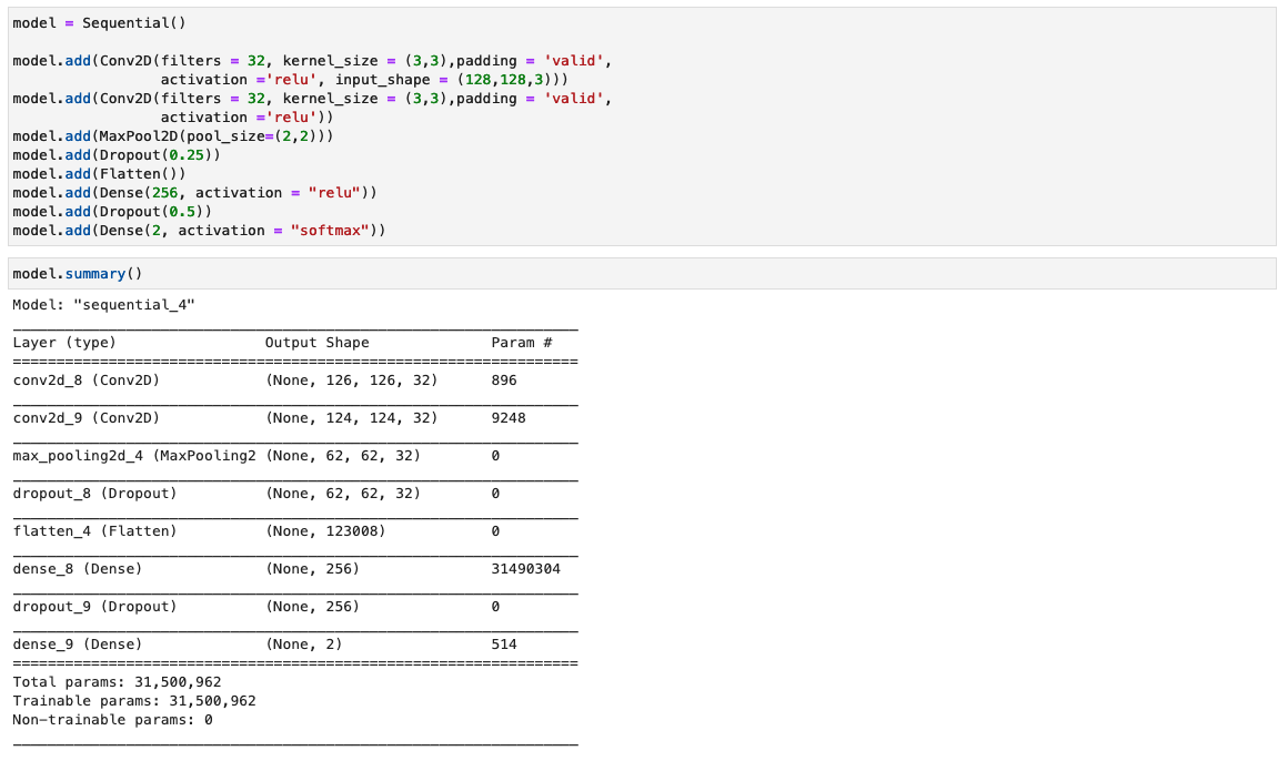
Note the following configurations:

Input – The model takes in an image input size of 128x128x3.
Convolutional layers – The convolutional layers use a minimal receptive field (3×3), the smallest possible size that still captures up/down and left/right. This is followed by a rectified linear unit (ReLU) activation function that reduces training time. This is a linear function that will output the input if positive; otherwise, the output is zero. The convolution stride is fixed at the default (1 pixel) to keep the spatial resolution preserved after convolution (stride is the number of pixel shifts over the input matrix).
Fully connected layers – The network has two fully connected layers. The first dense layer uses ReLU activation, and the second uses softmax to classify the image as original or tampered.

You can ignore any warnings when running these cells.

Save the model artifacts

Save the trained model with a unique file name—for example, based on the current date and time—into a directory named model.

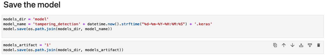
Save the tensorflow model artifacts

The model is saved in Keras format with the extension .keras. We also save the model artifacts as a directory named 1 containing serialized signatures and the state needed to run them, including variable values and vocabularies to deploy to a SageMaker runtime (which we discuss later in this post).

Measure model performance

The following loss curve shows the progression of the model’s loss over training epochs (iterations).

model accuracy plot

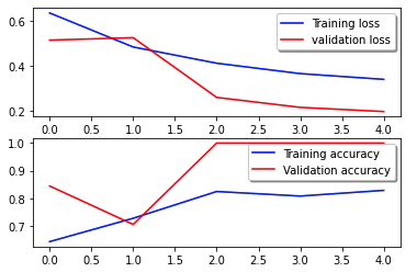
The loss function measures how well the model’s predictions match the actual targets. Lower values indicate better alignment between predictions and true values. Decreasing loss over epochs signifies that the model is improving. The accuracy curve illustrates the model’s accuracy over training epochs. Accuracy is the ratio of correct predictions to the total number of predictions. Higher accuracy indicates a better-performing model. Typically, accuracy increases during training as the model learns patterns and improves its predictive ability. These will help you determine if the model is overfitting (performing well on training data but poorly on unseen data) or underfitting (not learning enough from the training data).

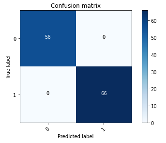
The following confusion matrix visually represents how well the model accurately distinguishes between the positive (forged image, represented as value 1) and negative (untampered image, represented as value 0) classes.

Confusion matrix plot

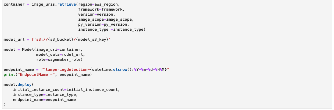
Following the model training, our next step involves deploying the computer vision model as an API. This API will be integrated into business applications as a component of the underwriting workflow. To achieve this, we use Amazon SageMaker Inference, a fully managed service. This service seamlessly integrates with MLOps tools, enabling scalable model deployment, cost-efficient inference, enhanced model management in production, and reduced operational complexity. In this post, we deploy the model as a real-time inference endpoint. However, it’s important to note that, depending on the workflow of your business applications, the model deployment can also be tailored as batch processing, asynchronous handling, or through a serverless deployment architecture.

Set up the model deployment notebook

Complete the following steps to set up your model deployment notebook:

Open the tampering_detection_model_deploy.ipynb file from document-tampering-detection directory.
Set up the notebook environment with the image Data Science 3.0.
For Kernel, choose Python3.
For Instance type, choose ml.t3.medium.

With an ml.t3.medium notebook environment, the cost per hour is $0.056 USD.

Create a custom inline policy for the SageMaker role to allow all Amazon S3 actions

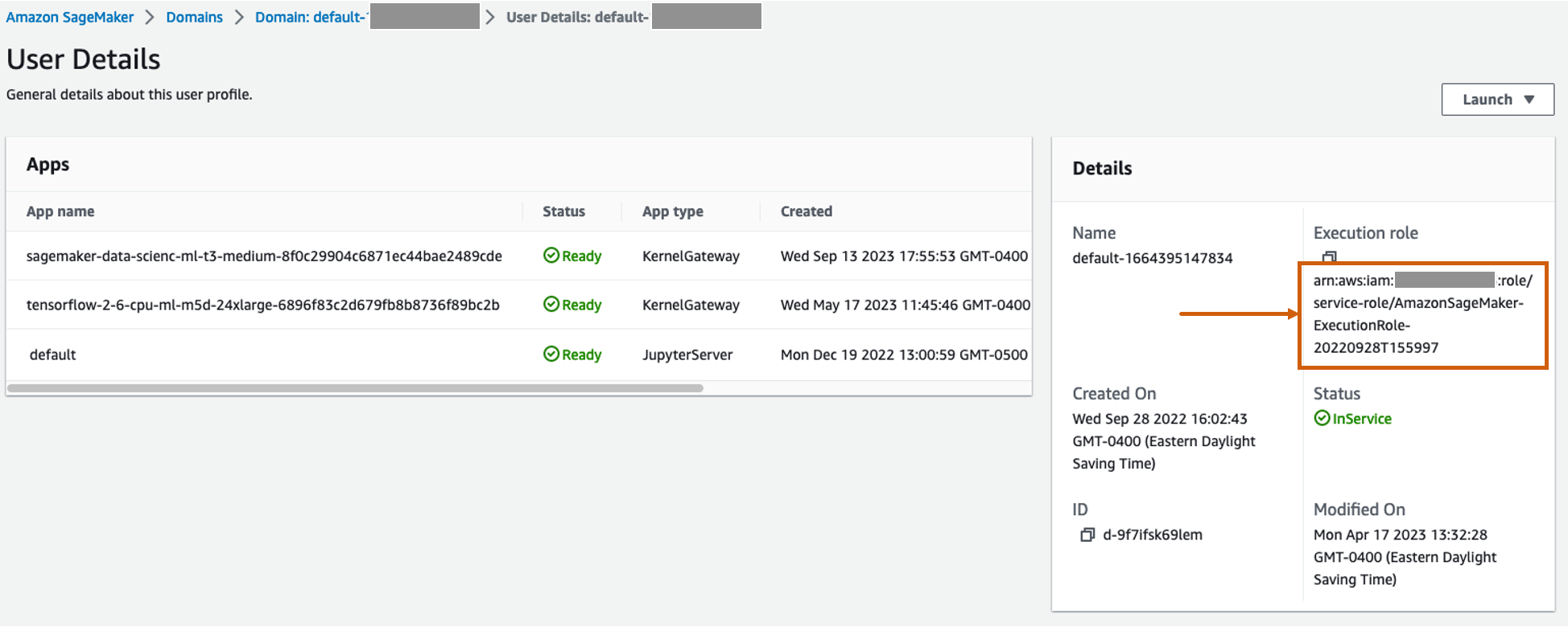
The AWS Identity and Access Management (IAM) role for SageMaker will be in the format AmazonSageMaker- ExecutionRole-<random numbers>. Make sure you’re using the correct role. The role name can be found under the user details within the SageMaker domain configurations.

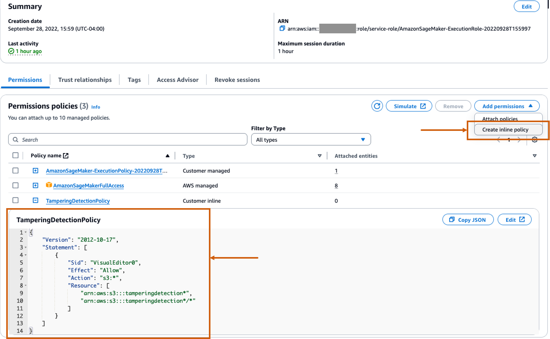
Update the IAM role to include an inline policy to allow all Amazon Simple Storage Service (Amazon S3) actions. This will be required to automate the creation and deletion of S3 buckets that will store the model artifacts. You can limit the access to specific S3 buckets. Note that we used a wildcard for the S3 bucket name in the IAM policy (tamperingdetection*).

Run the deployment notebook

Run each cell in the notebook tampering_detection_model_deploy.ipynb in order. We discuss some cells in more detail in the following sections.

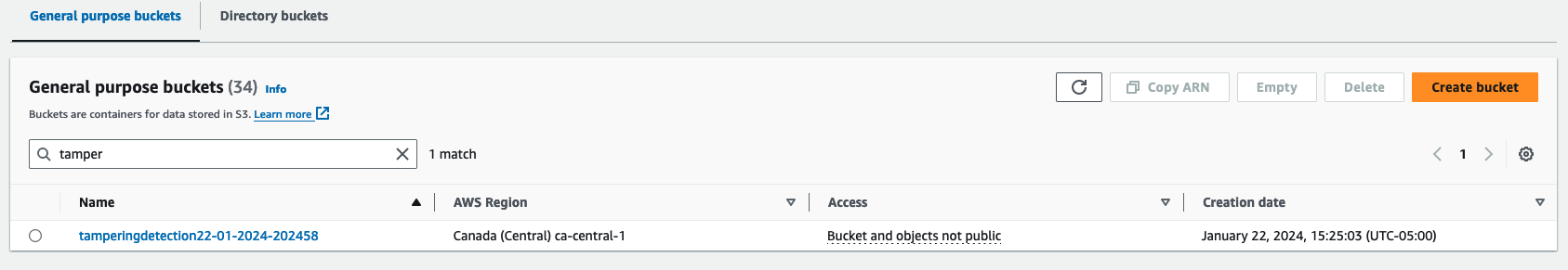
Create an S3 bucket

Run the cell to create an S3 bucket. The bucket will be named tamperingdetection<current date time> and in the same AWS Region as your SageMaker Studio environment.

Create Amazon S3 bucket

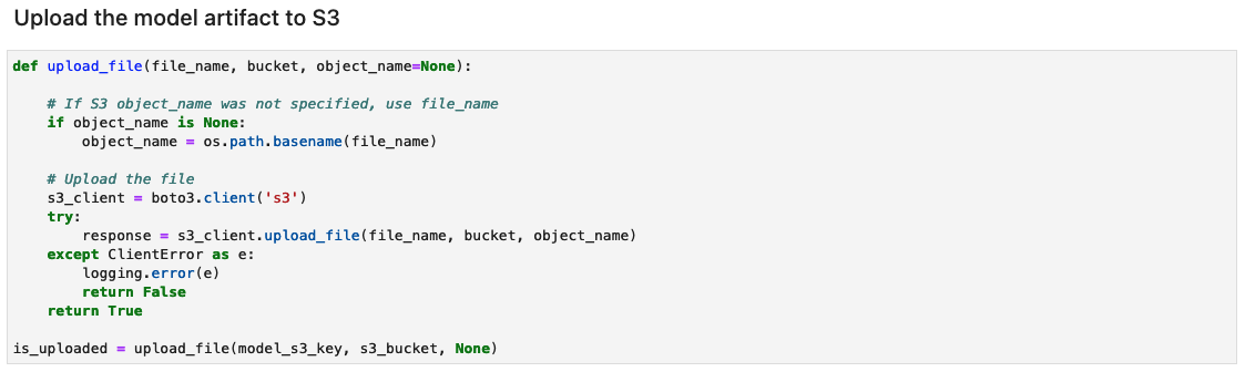
Create the model artifact archive and upload to Amazon S3

Create a tar.gz file from the model artifacts. We have saved the model artifacts as a directory named 1, containing serialized signatures and the state needed to run them, including variable values and vocabularies to deploy to the SageMaker runtime. You can also include a custom inference file called inference.py within the code folder in the model artifact. The custom inference can be used for preprocessing and postprocessing of the input image.

Upload model artifacts to Amazon S3

Create a SageMaker inference endpoint

The cell to create a SageMaker inference endpoint may take a few minutes to complete.

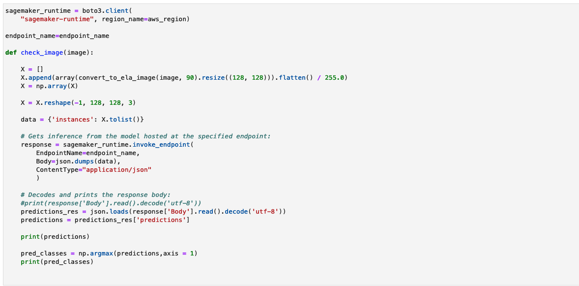
Create Amazon SageMaker Inference endpoint

Test the inference endpoint

The function check_image preprocesses an image as an ELA image, sends it to a SageMaker endpoint for inference, retrieves and processes the model’s predictions, and prints the results. The model takes a NumPy array of the input image as an ELA image to provide predictions. The predictions are output as 0, representing an untampered image, and 1, representing a forged image.

Test Amazon SageMaker Inference endpoint

Let’s invoke the model with an untampered image of a paystub and check the result.

Test an original image

The model outputs the classification as 0, representing an untampered image.

Now let’s invoke the model with a tampered image of a paystub and check the result.

Test a forged image

The model outputs the classification as 1, representing a forged image.

Limitations

Although ELA is an excellent tool for helping detect modifications, there are a number of limitations, such as the following:

A single pixel change or minor color adjustment may not generate a noticeable change in the ELA because JPEG operates on a grid.
ELA only identifies what regions have different compression levels. If a lower-quality image is spliced into a higher-quality picture, then the lower-quality image may appear as a darker region.
Scaling, recoloring, or adding noise to an image will modify the entire image, creating a higher error level potential.
If an image is resaved multiple times, then it may be entirely at a minimum error level, where more resaves do not alter the image. In this case, the ELA will return a black image and no modifications can be identified using this algorithm.
With Photoshop, the simple act of saving the picture can auto-sharpen textures and edges, creating a higher error level potential. This artifact doesn’t identify intentional modification; it identifies that an Adobe product was used. Technically, ELA appears as a modification because Adobe automatically performed a modification, but the modification was not necessarily intentional by the user.

We recommend using ELA alongside other techniques previously discussed in the blog in order to detect a greater range of image manipulation cases. ELA can also serve as an independent tool for visually examining image disparities, especially when training a CNN-based model becomes challenging.

Clean up

To remove the resources you created as part of this solution, complete the following steps:

Run the notebook cells under the Cleanup section. This will delete the following:
1. SageMaker inference endpoint – The inference endpoint name will be tamperingdetection-<datetime>.
2. Objects within the S3 bucket and the S3 bucket itself – The bucket name will be tamperingdetection<datetime>.
Shut down the SageMaker Studio notebook resources.

Conclusion

In this post, we presented an end-to-end solution for detecting document tampering and fraud using deep learning and SageMaker. We used ELA to preprocess images and identify discrepancies in compression levels that may indicate manipulation. Then we trained a CNN model on this processed dataset to classify images as original or tampered.

The model can achieve strong performance, with an accuracy over 95% with a dataset (forged and original) suited for your business requirements. This indicates that it can reliably detect forged documents like paystubs and bank statements. The trained model is deployed to a SageMaker endpoint to enable low-latency inference at scale. By integrating this solution into mortgage workflows, institutions can automatically flag suspicious documents for further fraud investigation.

Although powerful, ELA has some limitations in identifying certain types of more subtle manipulation. As next steps, the model could be enhanced by incorporating additional forensic techniques into training and using larger, more diverse datasets. Overall, this solution demonstrates how you can use deep learning and AWS services to build impactful solutions that boost efficiency, reduce risk, and prevent fraud.