AWS Partner Network (APN) Blog
Improving Dataset Query Time and Maintaining Flexibility with Amazon Athena and Amazon Redshift
By Matt Yellen, Principal Engineer at CloudZero
 |
 |
Analyzing large datasets can be challenging, especially if you aren’t thinking about certain characteristics of the data and what you’re ultimately looking to achieve.
There are a number of factors organizations need to consider in order to build systems that are flexible, affordable, and fast, while at the same time meeting the needs of their end users.
For example, you need to understand where your data is coming from, how often it changes, and how the data will be queried. In some cases, a fixed one-time analysis will be sufficient, while in other cases you’ll need to explore the data with dynamic ad-hoc queries.
Amazon Web Services (AWS) offers various data tools that serve different use cases and meet different needs for companies. Amazon Athena is a serverless, interactive query service that makes it easy to analyze data using standard SQL. Amazon Redshift is a cloud data warehouse that enables users to gain new insights from their data.
At CloudZero, an AWS Partner Network (APN) Advanced Technology Partner, I have used Amazon Athena, Amazon Redshift, and Amazon Redshift Spectrum to analyze our customers’ billing data.
Through this process, I have learned about the different capabilities of these AWS data services and which use cases they are best applied to.
In this post, I will walk you through how we used these AWS services to analyze customer billing data and provide value to end users.
Step 1: Getting the Data into Amazon S3
CloudZero is a platform that ingests billing data from AWS, as well as information about engineering activity and resources, in order to provide customers with insights about their costs and what caused them.
This requires us to build systems that work for customers’ unique environments, costs, and key performance indicators (KPI). The solution needed to offer flexible ways to group, filter, and partition the data. It also needed to be fast.
Before you can start analyzing the data, you need to get access to it. In our case, the data we needed was from the AWS Cost and Usage Report. For a customer’s monthly bill, we needed the complete set of things for which they were charged.
This includes resources like AWS Lambda, Amazon Elastic Compute Cloud (Amazon EC2) instances, or Amazon Simple Storage Service (Amazon S3) buckets; operations like data transfer or storage costs; and API usage like querying Amazon CloudWatch metrics.
For each charge, we also required a number of attributes so our customers would be able to group and filter this data in ways meaningful to their business. This included, for example, the account the charge applied to, AWS services used, resource ID (if applicable), operational metrics such as product family or usage type, and any tags (both AWS tags and customer user tags) applied to these resources.
We also wanted to access any other attributes associated with the changes for research purposes. For any particular change, there may be dozens, if not hundreds, of different attributes that may be valuable.
We directed the AWS Cost and Usage Report to be sent to an Amazon S3 bucket. The reports are delivered to S3 up to three times a day throughout the billing period, with each report replacing the last until they are finalized at the end of the month.
Next, we gave our report a name and specified the contents. Since we were looking to examine cost data down to an individual resource, we included resource IDs in the report. To ensure we had the most up-to-date data, we set the report to automatically refresh previous months.
We then specified an S3 bucket where the report should be placed, and we used hourly granularity so that customers could get the most detailed cost insights.
Step 2: Analyzing the Data with Amazon Athena
Once we configured regular billing drops from the AWS Cost and Usage Report, we were able to start analyzing the data using Amazon Athena.
For our use case, we needed something that was highly performant and supported ad-hoc queries.
Athena provided a number of advantages for our use case, including:
- Support for ad hoc queries: Athena uses Presto as its database engine and allowed us to query the data using standard SQL.
- Easy to set up: The AWS Cost and Usage Report produces parquet files that are queried directly by Athena; no additional extract, transform, and load (ETL) steps are required. It also provides an AWS CloudFormation template for an AWS Glue crawler to create the necessary schema.
- Serverless: There are no machines to configure or virtual private clouds (VPC) to manage.
- Secure: Access is controlled through AWS Identity and Access Management (IAM) policies so there’s no need to manage username or password credentials.
- Inexpensive: Data is stored and directly queried from an Amazon S3 bucket. You only pay for the queries that are run based on the amount of data scanned.
- Speed: Query performance is excellent, especially when using queries that take advantage of the partitioned parquet files produced by the AWS Cost and Usage Report.
In order to start using Athena, we needed to create the schema that represents our billing data. Fortunately, this can be done automatically by AWS Glue, a fully managed ETL service that makes it easy to prepare and load data for analytics.
To make things even easier, the AWS Cost and Billing Report provides a CloudFormation template to configure the AWS Glue crawler.
The crawler-cfn.yml file was available inside the S3 bucket we set up for the reports, and once that was downloaded we used CloudFormation to create a new stack and then uploaded the template file.
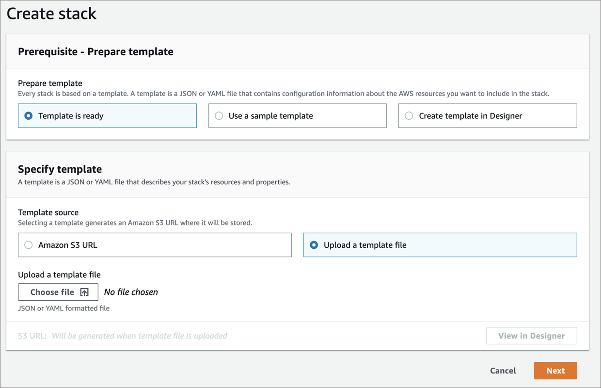
Figure 1 – Uploading the AWS CloudFormation template.
The template created the AWS Glue crawler and database, IAM roles needed for access, and Lambda function to start the crawler. It also created an S3 notification to invoke that Lambda function each time the billing report is updated.
Once the crawler runs, it creates a table we can immediately query from the Athena console, or do so programmatically.
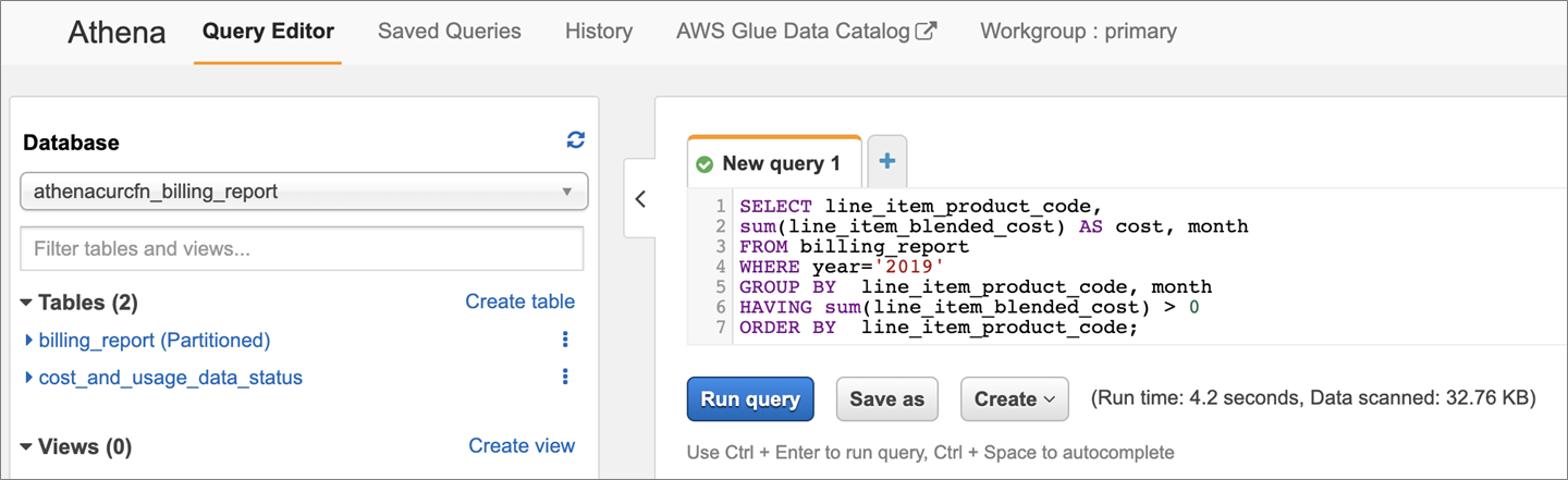
Figure 2 – Querying the table from the Amazon Athena console.
For example, this is a view of costs broken down by service and months in 2019:
Note the use of the columns “year” and “month,” which are the partition columns automatically generated by the AWS Glue crawler. Using them allows Athena to restrict the query to specific parquet files, reducing the amount of data that needs to be scanned.
This dramatically improves query performance and reduces cost. Partition columns should be used in your queries whenever possible.
Step 3: Creating External Tables with Amazon Redshift Spectrum
Once we had set up Amazon Athena to analyze our data, we started to plan how we would scale it up for the number of customers we were planning to support. At any given time, we needed Athena to allow hundreds of users to examine their cost data.
In addition, we planned to implement automated analysis of this data to reveal and report on cost anomalies, but we realized these queries could take tens of minutes to run. This revealed one challenge we faced using Athena: concurrency.
By default, Athena only supports 20 concurrent queries. Although you can request an increase, it quickly became apparent this limit was going to be a problem for us. The solution: Amazon Redshift Spectrum.
Amazon Redshift Spectrum isn’t really a separate AWS service, but rather a feature of Amazon Redshift itself. It allows a user to create “external” tables, which can be queried just like normal tables but are backed by am AWS Glue schema and S3 file, just like with Athena.
Amazon Redshift supports vastly more concurrent queries than Athena. In fact, by enabling features such as Concurrency Scaling, the number of possible concurrent queries is functionally infinite.
Setting up an Amazon Redshift cluster meant we lost some of the setup advantages of Athena. Unlike with Athena, though, our team now had some infrastructure to create and maintain.
The procedure for creating the Amazon Redshift cluster is outside the scope of this post, but once the cluster was ready we used the following SQL statement to configure the location of the billing data in Athena:
You may notice we didn’t actually create an external table, but rather an external schema and pointed it at the AWS Glue database. This ensures that if we ever update the AWS Glue crawler to create additional tables, they will immediately be available in Amazon Redshift.
Here’s an example of a simple query: total cost, grouped by service, for all of 2019. Note this is the Amazon Redshift query, and that the syntax is slightly different in Athena but still functionally the same.
We then tested this query with both Amazon Redshift Spectrum and Amazon Athena, to determine the difference in execution time.
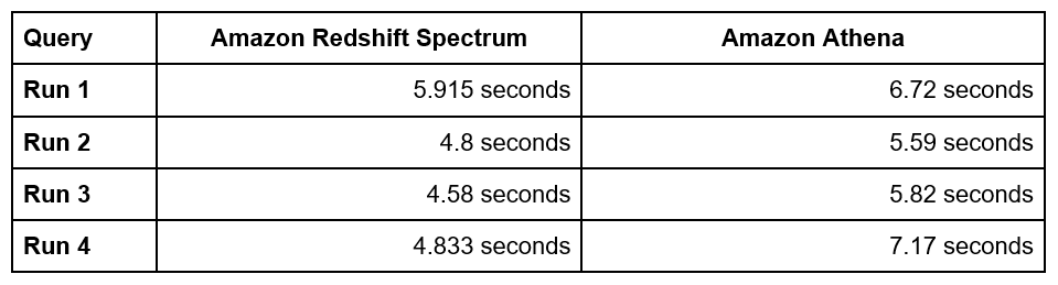
Figure 3 – Query time results from Amazon Redshift Spectrum and Amazon Athena.
For our configuration, Amazon Redshift is slightly faster, but we needed something faster to power an interactive dashboard.
Amazon Redshift has a really good result cache, so we expected subsequent queries to be nearly instantaneous. However, it seems that external tables don’t take advantage of that.
Also, the primary use case for our dashboard is to view cost data grouped by day, or by account/service over a time period with daily granularity. We should be able to get better performance by pre-aggregating the data and generating a new table.
We knew this would sacrifice some query flexibility, but we could always fall back to querying the external tables for less common use cases.
Step 4: Building Optimized Tables in Amazon Redshift
Our next step was to build a new table optimized for our most common use cases: daily granularity with the ability to filter and group by account and service.
That did the trick, so we took that query and turned it into a materialized view. Amazon Redshift doesn’t actually support materialized views, but it does have the next best thing: “CREATE TABLE AS”.
This command allowed us to create new tables from any query:
With that, we had a new “cost_by_day” table with four columns aggregated by service, account, and day.
Although querying this table was much faster, we thought we could do even better. Our dashboard allows filtering and grouping by product_code, usage_account_id, and usage_day columns.
By specifying a sortkey when creating the new table, you can tell Amazon Redshift to sort all the data by that column, dramatically reducing the amount of data it needs to scan during a group or filter operation.
Since we almost always want to filter by day (more recent data is generally more interesting), we used that first and followed with usage_account_id and product_code.
Next, we tested some queries. Here’s the same query we ran before, but modified to work with the new table:
To make this a fair test, we even disabled the Amazon Redshift result cache for our session. That ensured the query actually executes on the cluster every time we run it.
So, how does the new query compare the ones we ran against Amazon Athena and the Amazon Redshift Spectrum external table? As you can see below, the query times were about 50 times faster, but what about generating the optimized table itself?

Figure 4 – Comparison of query times with new Amazon Redshift optimized table using CloudZero billing data.
So far, we had been using CloudZero’s billing data for these tests. We have data going back to July 2018, and it consists of about 50 million line items totaling 6.8 GB. Generating the optimized Amazon Redshift table on that data set completed in 6.68 seconds.
Next, we wanted to try it on a much larger set. One of the largest bills CloudZero manages consists of about 1.9 billion line items and a total of 291 GB of data. Generating that optimized table completed in only 44 seconds.
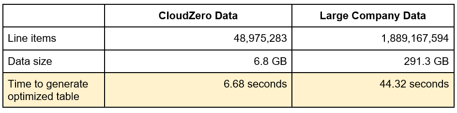
Figure 5 – Results of test with large enterprise customer.
At these speeds, there’s no need to update the optimized tables; we can just drop and recreate them every time we get new billing data.
Results
The architecture we’ve created has produced a number of benefits for both our engineering team and customers. By using AWS Glue to automatically analyze billing parquet files in Amazon S3, we avoided having to build and maintain our own complex ETL process.
Our engineering team doesn’t have to be concerned with differences between customer billing data schemas, or changes to the schemas over time. Updates to table schemas are handled automatically and transparently by the AWS Glue crawler.
In addition, Amazon Redshift Spectrum allows access to the complete set of billing data with simple SQL queries. This allows our data science team to explore the data and develop and test new algorithms. This enables our team to constantly innovate and develop new ways to detect anomalies and group costs.
Amazon Redshift Spectrum has also made it easy to generate new Amazon Redshift tables by pre-aggregating the data and performing some expensive calculations up front. Since new tables can be created from SQL queries, there’s no need for the engineering team to maintain additional code.
This has the added advantage of easily scaling up as we add more and more large customers. Since Amazon Redshift automatically distributes queries across all nodes in the cluster, as we grow, we simply need to add more nodes.
The tables generated from this process allowed us to build an extremely responsive and flexible dashboard. Even as we’ve added new options for grouping and filtering data, we’ve experienced almost no degradation in performance. This has proven incredibly valuable as we explore even more complex relationships between resources for establishing cost groups.
Summary
In this post, we looked at techniques for analyzing a large data set—in this case, AWS billing data—using Amazon Athena, Amazon Redshift, and Amazon Redshift Spectrum.
CloudZero is a cost management solution that provides a new perspective into companies’ cloud spend by correlating billing data with engineering activity.
To build a product that was effective, performant, and flexible, we started with Athena and found it was a good choice for ease of setup and management, low cost, and performance.
Our use case required more concurrent connections, however, and we solved for this by using Amazon Redshift Spectrum, which allows AWS customers to query their data in Amazon S3. We created external tables in our Amazon Redshift cluster and pointed them at the existing tables in Athena to ensure they stayed up to date.
Finally, to get an additional performance boost for our most common use cases, we leveraged Amazon Redshift’s “CREATE TABLE AS” command to produce new optimized tables.
This operation was fast enough to simply re-run every time we receive new billing data and provided a 50X increase in the speed of our queries, as shown in the tables above.
To learn more about CloudZero, visit cloudzero.com and get started with a free trial.
The content and opinions in this blog are those of the third party author and AWS is not responsible for the content or accuracy of this post.
.

.
CloudZero – APN Partner Spotlight
CloudZero is an APN Advanced Technology Partner. Its solution eliminates cost surprises and improves efficiency and resource usage, helping organizations to innovate at a faster rate.
Contact CloudZero | Solution Overview | AWS Marketplace
*Already worked with CloudZero? Rate this Partner
*To review an APN Partner, you must be an AWS customer that has worked with them directly on a project.