Artificial Intelligence
AWS Inferentia2 builds on AWS Inferentia1 by delivering 4x higher throughput and 10x lower latency
The size of the machine learning (ML) models––large language models (LLMs) and foundation models (FMs)––is growing fast year-over-year, and these models need faster and more powerful accelerators, especially for generative AI. AWS Inferentia2 was designed from the ground up to deliver higher performance while lowering the cost of LLMs and generative AI inference.
In this post, we show how the second generation of AWS Inferentia builds on the capabilities introduced with AWS Inferentia1 and meets the unique demands of deploying and running LLMs and FMs.
The first generation of AWS Inferentia, a purpose-built accelerator launched in 2019, is optimized to accelerate deep learning inference. AWS Inferentia helped ML users reduce their inference costs and improve their prediction throughput and latency. With AWS Inferentia1, customers saw up to 2.3x higher throughput and up to 70% lower cost per inference than comparable inference-optimized Amazon Elastic Compute Cloud (Amazon EC2) instances.
AWS Inferentia2, featured in the new Amazon EC2 Inf2 instances and supported in Amazon SageMaker, is optimized for large-scale generative AI inference and is the first inference focused instance from AWS that is optimized for distributed inference, with high-speed, low-latency connectivity between accelerators.
You can now efficiently deploy a 175-billion-parameter model for inference across multiple accelerators on a single Inf2 instance without requiring expensive training instances. Until now, customers who had large models could only use instances that were built for training, but this is a waste of resources––given that they’re more expensive, consume more energy, and their workload doesn’t make use of all the available resources (such as faster networking and storage). With AWS Inferentia2, you can achieve 4 times higher throughput and up to 10 times lower latency compared to AWS Inferentia1. Also, the second generation of AWS Inferentia adds enhanced support for more data types, custom operators, dynamic tensors, and more.
AWS Inferentia2 has 4 times more memory capacity, 16.4 times higher memory bandwidth than AWS Inferentia1, and native support for sharding large models across multiple accelerators. The accelerators use NeuronLink and Neuron Collective Communication to maximize the speed of data transfer between them or between an accelerator and the network adapter. AWS Inferentia2 is better suited for larger models, which require sharding across multiple accelerators, although AWS Inferentia1 is still a great option for smaller models because it provides better price-performance compared to alternatives.
Architecture evolution
To compare both generations of AWS Inferentia, let’s review the architecture of AWS Inferentia1. It has four NeuronCores v1 per chip, shown in the following diagram.

Specifications per chip:
- Compute – Four cores delivering in total 128 INT8 TOPS and 64FP16/BF16 TFLOPS
- Memory – 8 GB of DRAM (50 GB/sec of bandwidth), shared by all four cores
- NeuronLink – Link between cores for sharding models across two or more cores
Let’s look at how AWS Inferentia2 is organized. Each AWS Inferentia2 chip has two upgraded cores based on the NeuronCore-v2 architecture. Like AWS Inferentia1, you can run different models on each NeuronCore or combine multiple cores to shard big models.
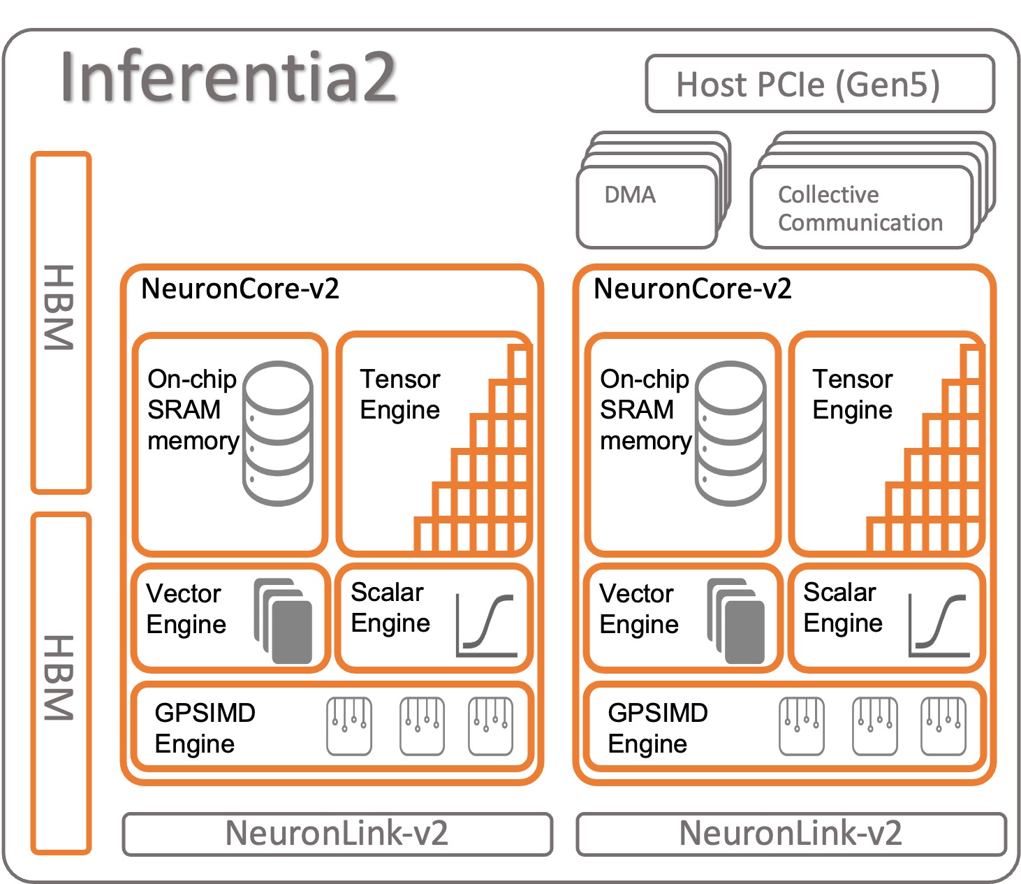
Specifications per chip:
- Compute – Two cores delivering in total 380 INT8 TOPS, 190 FP16/BF16/cFP8/TF32 TFLOPS, and 47.5 FP32 TFLOPS
- Memory – 32 GB of HBM, shared by both cores
- NeuronLink – Link between chips (384 GB/sec per device) for sharding models across two or more cores
NeuronCore-v2 has a modular design with four independent engines:
- ScalarEngine (3 times faster than v1) – Operates on floating point numbers––1600 (BF16/FP16) FLOPS
- VectorEngine (10 times faster than v1) – Operates on vectors of numbers with single operation for computations such as normalization, pooling, and others.
- TensorEngine (6 times faster than v1) – Performs tensor computations such as Conv, Reshape, Transpose, and others.
- GPSIMD-Engine – Has eight fully programmable 512-bit wide general-purpose processors for you to create your custom operators with standard PyTorch custom C++ operators API. This is a new feature, introduced in NeuronCore-v2.
AWS Inferentia2 NeuronCore-v2 is faster and more optimized. Also, it’s capable of accelerating different types and sizes of models, ranging from simple models such as ResNet 50 to large language models or foundation models with billions of parameters such as GPT-3 (175 billion parameters). AWS Inferentia2 also has a larger and faster internal memory, when compared to AWS Inferentia1, as shown in the following table.
| Chip | Neuron Cores | Memory Type | Memory Size | Memory Bandwidth |
| AWS Inferentia | x4 (v1) | DDR4 | 8GB | 50GB/S |
| AWS Inferentia 2 | x2 (v2) | HBM | 32GB | 820GB/S |
The memory you find in AWS Inferentia2 is the type High-Bandwidth Memory (HBM) type. Each AWS Inferentia2 chip has 32 GB and that can be combined with other chips to distribute very large models using NeuronLink (device-to-device interconnect). An inf2.48xlarge, for instance, has 12 AWS Inferentia2 accelerators with a total of 384 GB of accelerated memory. The speed of AWS Inferentia2 memory is 16.4 times faster than AWS Inferentia1, as shown in the previous table.
Other features
AWS Inferentia2 offers the following additional features:
- Hardware supported – cFP8 (new, configurable FP8), FP16, BF16, TF32, FP32, INT8, INT16 and INT32. For more information, refer to Data Types.
- Lazy Tensor inference – We discuss Lazy Tensor inference later in this post.
- Custom operators – Developers can use standard PyTorch custom operators programming interfaces to use the Custom C++ Operators feature. A custom operator is composed of low-level primitives available in the Tensor Factory Functions and accelerated by GPSIMD-Engine.
- Control-flow (coming soon) – This is for native programming language control flow inside the model to eventually preprocess and postprocess data from one layer to another.
- Dynamic-shapes (coming soon) – This is useful when your model changes the shape of the output of any internal layer dynamically. For instance: a filter which reduces the output tensor size or shape inside the model, based on the input data.
Accelerating models on AWS Inferentia1 and AWS Inferentia2
The AWS Neuron SDK is used for compiling and running your model. It is natively integrated with PyTorch and TensorFlow. That way, you don’t need to run an additional tool. Use your original code, written in one of these ML frameworks, and with a few lines of code changes, you’re good to go with AWS Inferentia.
Let’s look at how to compile and run a model on AWS Inferentia1 and AWS Inferentia2 using PyTorch.
Load a pre-trained model (ResNet 50) from torchvision
Load a pre-trained model and run it one time to warm it up:
Trace and deploy the accelerated model on Inferentia1
To trace the model to AWS Inferentia, import torch_neuron and invoke the tracing function. Keep in mind that the model needs to be PyTorch Jit traceable to work.
At the end of the tracing process, save the model as a normal PyTorch model. Compile the model one time and load it back as many times as you need. The Neuron SDK runtime is already integrated to PyTorch and is responsible for sending the operators to the AWS Inferentia1 chip automatically to accelerate your model.
In your inference code, you always need to import torch_neuron to activate the integrated runtime.
You can pass additional parameters to the compiler to customize the way it optimizes the model or to enable special features such as neuron-pipeline-cores. Shard your model across multiple cores to increase throughput.
Tracing and deploying the accelerated model on Inferentia2
For AWS Inferentia2, the process is similar. The only difference is the package you import ends with x: torch_neuronx. The Neuron SDK takes care of the compilation and running of the model for you transparently. You can also pass additional parameters to the compiler to fine-tune the operation or activate specific functionalities.
AWS Inferentia2 also offers a second approach for running a model called Lazy Tensor inference. In this mode, you don’t trace or compile the model previously; instead, the compiler runs on the fly every time you run your code. It isn’t recommended for production, given that traced mode has many advantages over Lazy Tensor inference. However, if you’re still developing your model and need to test it faster, Lazy Tensor inference can be a good alternative. Here’s how to compile and run a model using Lazy Tensor:
Now that you’re familiar with AWS Inferentia2, a good next step is to get started with PyTorch or Tensorflow and learn how to set up a dev environment and run tutorials and examples. Also, check the AWS Neuron Samples GitHub repo, where you can find multiple examples of how to prepare models to run on Inf2, Inf1, and Trn1.
Summary of feature comparison between AWS Inferentia1 and AWS Inferentia2
The AWS Inferentia2 compiler is XLA-based, and AWS is part of OpenXLA initiative. This is the biggest difference over AWS Inferentia1, and that’s relevant because PyTorch, TensorFlow, and JAX have native XLA integrations. XLA brings many performance improvements, given that it optimizes the graph to compute the results in a single kernel launch. It fuses together successive tensor operations and outputs optimal machine code for accelerating model runs on AWS Inferentia2. Other parts of the Neuron SDK were also improved in AWS Inferentia2, while keeping the user experience as simple as possible while tracing and running models. The following table shows the features available in both versions of the compiler and runtime.
| Feature | torch-neuron | torch-neuronx |
| Tensorboard | Yes | Yes |
| Supported Instances | Inf1 | Inf2 & Trn1 |
| Inference Support | Yes | Yes |
| Training Support | No | Yes |
| Architecture | NeuronCore-v1 | NeuronCore-v2 |
| Trace API | torch_neuron.trace() | torch_neuronx.trace() |
| Distributed inference | NeuronCore Pipeline | Collective Communications |
| IR | GraphDef | HLO |
| Compiler | neuron-cc | neuronx-cc |
| Monitoring | neuron-monitor / monitor-top | neuron-monitor / monitor-top |
For a more detailed comparison between torch-neuron (Inf1) and torch-neuronx (Inf2), refer to Comparison of torch-neuron (Inf1) versus torch-neuronx (Inf2 & Trn1) for Inference.
Model Serving
After tracing a model to deploy to Inf2, you have many deployment options. You can run real-time predictions or batch predictions in different ways. Inf2 is available because EC2 instances are natively integrated to other AWS services that make use of Deep Learning Containers (DLCs) such as Amazon Elastic Container Service (Amazon ECS), Amazon Elastic Kubernetes Service (Amazon EKS), and SageMaker.
AWS Inferentia2 is compatible with the most popular deployment technologies. Here are a list of some of the options you have for deploying models using AWS Inferentia2:
- SageMaker – Fully managed service to prepare data and build, train, and deploy ML models
- TorchServe – PyTorch integrated deployment mechanism
- TensorFlow Serving – TensorFlow integrated deployment mechanism
- Deep Java Library – Open-source Java mechanism for model deployment and training
- Triton – NVIDIA open-source service for model deployment
Benchmark
The following table highlights the improvements AWS Inferentia2 brings over AWS Inferentia1. Specifically, we measure latency (how fast the model can make a prediction using each accelerator), throughput (how many inferences per second), and cost per inference (how much each inference costs in US dollars). The lower the latency in milliseconds and costs in US dollars, the better. The higher the throughput the better.
Two models were used in this process––both large language models: ELECTRA large discriminator and BERT large uncased. PyTorch (1.13.1) and Hugging Face transformers (v4.7.0), the main libraries used in this experiment, ran on Python 3.8. After compiling the models for batch size = 1 and 10 (using the code from the previous section as a reference), each model was warmed up (invoked one time to initialize the context) and then invoked 10 times in a row. The following table shows average numbers collected in this simple benchmark.
- Electra large discriminator (334,092,288 parameters ~593 MB)
- Bert large uncased (335,143,938 parameters ~580 MB)
- OPT-66B (66 billion parameterss ~124 GB)
| Model Name | Batch Size | Sentence Length | Latency (ms) | Improvements Inf2 over Inf1 (x Times) | Throughput (Inferences per Second) | Cost per Inference (EC2 us-east-1) ** | |||
| Inf1 | Inf2 | Inf1 | Inf2 | Inf1 | Inf2 | ||||
| ElectraLargeDiscriminator | 1 | 256 | 35.7 | 8.31 | 4.30 | 28.01 | 120.34 | $0.0000023 | $0.0000018 |
| ElectraLargeDiscriminator | 10 | 256 | 343.7 | 72.9 | 4.71 | 2.91 | 13.72 | $0.0000022 | $0.0000015 |
| BertLargeUncased | 1 | 128 | 28.2 | 3.1 | 9.10 | 35.46 | 322.58 | $0.0000018 | $0.0000007 |
| BertLargeUncased | 10 | 128 | 121.1 | 23.6 | 5.13 | 8.26 | 42.37 | $0.0000008 | $0.0000005 |
* c6a.8xlarge with 32 AMD Epyc 7313 CPU was used in this benchmark.
**EC2 Public pricing in us-east-1 on April 20: inf2.xlarge: $0.7582/hr; inf1.xlarge: $0.228/hr. Cost per inference considers the cost per element in a batch. (Cost per inference equals the total cost of model invocation/batch size.)
For additional information about training and inference performance, refer to Trn1/Trn1n Performance.
Conclusion
AWS Inferentia2 is a powerful technology designed for improving performance and reducing costs of deep learning model inference. More performant than AWS Inferentia1, it offers up to 4 times higher throughput, up to 10 times lower latency, and up to 50% better performance/watt than other comparable inference-optimized EC2 instances. In the end, you pay less, have a faster application, and meet your sustainability goals.
It’s simple and straightforward to migrate your inference code to AWS Inferentia2, which also supports a broader variety of models, including large language models and foundation models for generative AI.
You can get started by following the AWS Neuron SDK documentation to set up a development environment and start your accelerated deep learning project. To help you get started, Hugging Face has added Neuron support to their Optimum library, which optimizes models for faster training and inference, and they have many examples tasks ready to run on Inf2. Also, check our Deploy large language models on AWS Inferentia2 using large model inference containers to learn about deploying LLMs to AWS Inferentia2 using model inference containers. For additional examples, see the AWS Neuron Samples GitHub repo.
About the authors
 Samir Araújo is an AI/ML Solutions Architect at AWS. He helps customers creating AI/ML solutions which solve their business challenges using AWS. He has been working on several AI/ML projects related to computer vision, natural language processing, forecasting, ML at the edge, and more. He likes playing with hardware and automation projects in his free time, and he has a particular interest for robotics.