Artificial Intelligence
Create, train, and deploy a billion-parameter language model on terabytes of data with TensorFlow and Amazon SageMaker
The increasing size of language models has been one of the biggest trends in natural language processing (NLP) in recent years. Since 2018, we’ve seen unprecedented development and deployment of ever-larger language models, including BERT and its variants, GPT-2, T-NLG, and GPT-3 (175 billion parameters).
These models have pushed the boundaries of possible architectural innovations. We face several challenges when training large-scale deep learning models, especially the new wave of generative pre-trained transformers. These challenges include hardware limitations and trade-offs with computation and efficiency. To overcome these challenges of model and data parallelism, AWS offers a wide range of capabilities.
In this post, we introduce two main approaches: data parallelization and model parallelization using Amazon SageMaker, and discuss their pros and cons.
The model
For the language model, we use Transformers, introduced in the paper Attention Is All You Need. Transformers are deep learning models designed to deliberately avoid the pitfalls of RNNs by relying on a self-attention mechanism to draw global dependencies between input and output. The Transformer model architecture allows for significantly better parallelization and can achieve high performance in relatively short training time. Built on the success of Transformers, BERT, introduced in the paper BERT: Pre-training of Deep Bidirectional Transformers for Language Understanding, added bidirectional pre-training for language representation. Inspired by the Cloze task, BERT is pre-trained with masked language modeling (MLM), in which the model learns to recover the original words for randomly masked tokens. The BERT model is also pretrained on the next sentence prediction (NSP) task to predict if two sentences are in correct reading order. Since its advent in 2018, BERT and its variations have been widely used in language models.
We begin by creating two embedding layers for token and positional embedding. The input embeddings are the sum of the token embeddings and position embeddings.
Then we define a transformer decoder block with two sub-layers: a multi-head self-attention layer, and a simple fully connected feed-forward network followed by layer normalization and dropout:
Finally, we create our language model with the preceding embedding layer and transformer blocks:
Depending on your hyperparameters, you can scale this model from thousands of parameters to billions of parameters. The primary challenge with billion-parameter models is that you can’t host the model in one instance and need to distribute the model over several nodes for training and inference.
The dataset
In our experiments, we used the Pile dataset. The Pile is an 800 GiB English text dataset designed for training large-scale language models. It is created from 22 diverse and high-quality datasets, including both established NLP datasets and newly introduced ones.
The dataset is created from a variety of data sources, including books; GitHub repositories; webpages; chat logs; and medical, physics, math, computer science, and philosophy papers. Specifically, it uses the following sources: Pile-CC, PubMed Central, ArXiv, GitHub, the FreeLaw Project, Stack Exchange, the US Patent and Trademark Office, PubMed, Ubuntu, IRC, HackerNews, YouTube, PhilPapers, Books3, Project Gutenberg (PG-19), OpenSubtitles, English Wikipedia, DM Mathematics, EuroParl, the Enron Emails corpus, and NIH ExPorter. It also includes OpenWebText2 and BookCorpus2, which are extensions of the original OpenWebText and BookCorpus datasets, respectively. The diversity in data sources can improve the general cross-domain knowledge and consequently improve downstream generalization capabilities.
The primary challenge with this dataset is the sheer size; the dataset has 825 GiB of text, which translates into 4.2 TiB of preprocessed and compressed datapoints. Similar to the challenges we face with training and hosting the models, training a model with this dataset on a single instance will take a lot of time and isn’t practical.
Our solution is to break down the dataset into approximately 1 GiB chunks of data, load and preprocess the features in TensorFlow Dataset objects, and store them in Amazon Elastic File Service (Amazon EFS). TensorFlow datasets provide an easy-to-use and high-performance data pipeline that integrates well with our models. Amazon EFS is an easy-to-use service that enables us to build a shared file system that scales automatically as files are added and deleted. In addition, Amazon EFS is capable of bursting to higher throughput levels when needed, which is critical in our data and model training pipeline.
Next, we look into distributed training strategies to tackle these challenges.
Distributed training
In this project, we faced two challenges: scaling model size and data volume. Increasing the model size and number of trainable parameters may result in better accuracy, but there’s a limit to the model you can fit into a single GPU memory or even multiple GPUs in a single instance. In addition, bigger model sizes take more time to train.
You can tackle these challenges two different ways: data parallelism and model parallelism. With data parallelism, we perform Stochastic Gradient Descent (SGD) by distributing the records of a mini-batch over different devices to speed up the training. However, parallel data training comes with extra complexity of computing mini-batch gradient average with gradients from all devices, a step called AllReduce, which becomes harder as the training cluster is grown. While using data parallelism, we must be able to fit the model and a single datapoint in a device (CPU or GPU), which is a limiting factor in our experiments because the size of such a large model is much larger than the single GPU’s memory size.
Another solution is to use model parallelism, which splits the model over multiple devices. Model parallelism is the process of splitting a model up between multiple devices or nodes (such as GPU-equipped instances) and creating an efficient pipeline to train the model across these devices to maximize GPU utilization.
Data parallelization
Parallelizing the data is the most common approach to multiple GPUs or distributed training. You can batch your data, send it to multiple devices (each hosting a replicated model), then aggregate the results. We experimented with two packages for data parallelization: Horovod and the SageMaker distributed data parallel library.
Horovod is a distributed deep learning training framework for TensorFlow, Keras, PyTorch, and Apache MXNet. To use Horovod, we went through the following process:
- Initialize by running
hvd.init(). - Associate each device with a single process. The first process or worker is associated with the first device, the second process is associated with the second device, and so on.
- Adjust the learning rate based on the number of devices.
- Wrap the optimizer in
hvd.DistributedOptimizer. - Broadcast the initial variable states from the first worker with rank 0 to all other processes. This is necessary to ensure consistent initialization of all workers when training is started with random weights or restored from a checkpoint.
- Make sure that only device 0 can save checkpoints to prevent other workers from corrupting them.
The following is the training script:
The SageMaker data parallel library enables us to scale our training with near-linear efficiency, speeding up our training with minimal code changes. The library performs a custom AllReduce operation and optimizes device-to-device communication by fully utilizing AWS’s network infrastructure and Amazon Elastic Compute Cloud (Amazon EC2) instance topology. To use the SageMaker data parallel library, we went through the following process:
- Import and initialize
sdp.init(). - Associate each device with a single
smdistributed.dataparallelprocess withlocal_rank.sdp.tensorflow.local_rank()gives us the local rank of devices. The leader is rank 0, and workers are rank 1, 2, 3, and so on. - Adjust the learning rate based on the number of devices.
- Wrap
tf.GradientTapewithDistributedGradientTapeto performAllReduce. - Broadcast the initial model variables from the leader node to all the worker nodes.
- Make sure that only device 0 can save checkpoints.
Model parallelization
We can adjust the hyperparameters to keep the model small enough to train using a single GPU, or we can use model parallelism to split the model between multiple GPUs across multiple instances. Increasing a model’s number of trainable parameters can result in better accuracy, but there’s a limit to the maximum model size you can fit in a single GPU memory. We used the SageMaker distributed model parallel library to train our larger models. The steps are as follows:
- Import and initialize the library with
smp.init(). - The Keras model needs to inherit from smp.DistributedModel instead of the Keras Model class.
- Set
drop_remainder=Truein thetf.Dataset.batch()method to ensure that the batch size is always divisible by the number of microbatches. - Random operations in the data pipeline all need to use the same seed:
smp.dp_rank(), for example,shuffle(ds, seed=smp.dp_rank()). This ensures consistency of data samples across devices that hold different model partitions. - Forward and backward logic needs to be in a step function with
smp.stepdecoration. - Perform postprocessing on the outputs across microbatches using StepOutput methods such as
reduce_mean. Thesmp.stepfunction must have a return value that depends on the output ofsmp.DistributedModel.
The training script is as follows:
For a detailed guide to enable the TensorFlow training script for the SageMaker distributed model parallel library, refer to Modify a TensorFlow Training Script. For PyTorch, refer to Modify a PyTorch Training Script.
SageMaker Debugger
In the previous sections, we discussed how to optimize the training using model and data parallelization techniques. With Amazon SageMaker Debugger, we can now capture performance profiling information from our training runs to determine how much the training has improved. By default, Debugger captures system metrics for each SageMaker training job such as GPU, CPU utilization, memory, network, and I/O at a sampling interval of 500 milliseconds. We can access the data as follows:
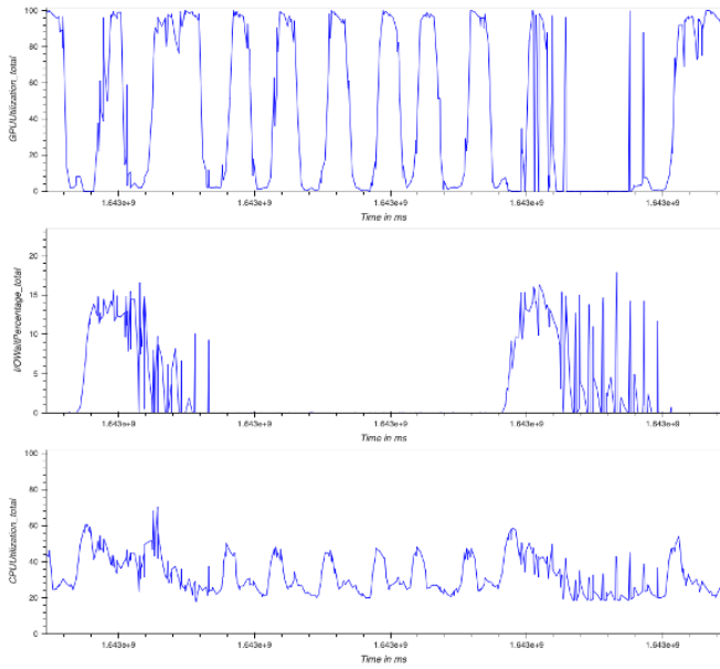
Debugger provides utilities to visualize the profiling data in different ways. In the following example, we see the total GPU and CPU utilization as well as the I/O wait time for the multi-GPU training job using Horovod. To generate these graphs, we run the following code:
The GPU utilization frequently fluctuates between 0–100%, and high I/O wait times with low GPU utilization are an indicator of an I/O bottleneck. Furthermore, the total CPU utilization never exceeds 70%, which means that we can improve data preprocessing by increasing the number of worker processes.
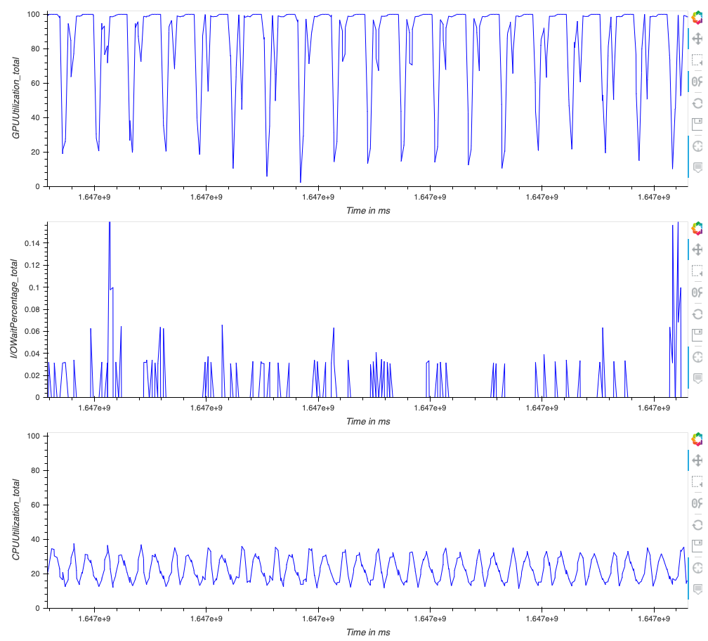
We can improve performance by switching from Horovod to the SageMaker distributed data parallel library. In the following graphs, we can see that GPUs are utilized more efficiently and only dropping to low utilization for short periods of time.
Training infrastructure
For training the models, we used 10 ml.p3.16xlarge instances using a SageMaker training job. SageMaker reduces the time and cost to train and tune machine learning (ML) models without the need to manage infrastructure. With SageMaker, you can easily train and tune ML models using built-in tools to manage and track training experiments, automatically choose optimal hyperparameters, debug training jobs, and monitor the utilization of system resources such as GPUs, CPUs, and network bandwidth. The data was hosted in Amazon EFS, which enabled us to grow and shrink as we add and remove files with no need for management or provisioning. Our primary objectives were to improve training speed and reduce costs.
Model scalability
Although this infrastructure is primarily used for language generation, with the GPT architecture and Pile dataset, you can use these techniques to train large-scale transformer models, which is useful in many domains beyond NLP. In machine learning itself, many computer vision tasks are now solved with large-parameter (transformer) architectures where they have been shown to outperform traditional CNNs (Convolutional Neural Network) on tasks like representation learning (see Advancing the state of the art in computer vision with self-supervised Transformers and 10x more efficient training) and large-scale mapping of images to text (such as CLIP). Large-parameter models are also breaking new ground in life sciences in fields like protein structure analysis and analysis of medical image data.
The solutions we detail in this post for distributed training and managing large models should apply to models in any of these domains as well.
Trade-offs
There has been an ongoing discussion in the research community regarding the risks of training large-scale language models, and whether enough thought has been put into the potential risks associated with developing them and strategies to mitigate these risks, some of which include the financial and environmental costs. According to a paper published in ACM, training a single BERT base model (without hyperparameter tuning) on GPUs was estimated to require as much energy as a trans-American flight. The environmental impacts scale with model size, and being able to efficiently fine-tune such models can potentially curtail the emissions significantly. AWS recently launched a new Customer Carbon Footprint Tool, available to all AWS customers at no cost, as part of Amazon’s efforts to increase sustainability and reduce carbon emissions. Running applications on the AWS Cloud can potentially decrease the carbon footprint (when compared to enterprise data centers that were surveyed in a 2019 report).
Conclusion
This post demonstrated a solution that facilitates the fine-tuning of language models with a billion parameters on the AWS Cloud using SageMaker.
For more information about model parallelism with SageMaker, refer to Train 175+ billion parameter NLP models with model parallel additions and Hugging Face on Amazon SageMaker and How Latent Space used the Amazon SageMaker model parallelism library to push the frontiers of large-scale transformers.
If you’d like help accelerating your use of ML in your products and processes, please contact the Amazon ML Solutions Lab.
About the Authors
 Sia Gholami is a Senior Data Scientist at the Amazon ML Solutions Lab, where he builds AI/ML solutions for customers across various industries. He is passionate about natural language processing (NLP) and deep learning. Outside of work, Sia enjoys spending time in nature and playing tennis.
 Mehdi Nooriis a Manager and a Senior Applied Scientist at the Amazon ML Solutions Lab, where he works with customers across various industries, and helps them to accelerate their cloud migration journey, and to solve their ML problems using state-of-the-art solutions and technologies.
 Muhyun Kim is a data scientist at Amazon Machine Learning Solutions Lab. He solves customer’s various business problems by applying machine learning and deep learning, and also helps them gets skilled.
 Danny Byrd is an Applied Scientist at the Amazon ML Solutions Lab. At the lab he’s helped customers develop advanced ML solutions, in ML specialties from computer vision to reinforcement learning. He’s passionate about pushing technology forward and unlocking new potential from AWS products along the way.
 Francisco Calderon Rodriguez is a Data Scientist in the Amazon ML Solutions Lab. As a member of the ML Solutions Lab, he helps solve critical business problems for AWS customers using deep learning. In his spare time, Francisco likes to play music and guitar, play soccer with his daughters, and enjoy time with his family.
 Yohei Nakayama is a Deep Learning Architect at the Amazon ML Solutions Lab. He works with customers across different verticals to accelerate their use of artificial intelligence and AWS Cloud services to solve their business challenges. He is interested in applying ML/AI technologies to the space industry.
 Nathalie Rauschmayr is a Senior Applied Scientist at AWS, where she helps customers develop deep learning applications.